PLC Datenlogger – User Manual
Overview
The PLC Datenlogger (PLC data logger) cyclically reads variables from one or several controllers of different manufacturers at the same time, stores all measurements in a common CSV file (and/or a database) and displays them as a y-t chart – in the user interface, in the browser (web server) or not at all (headless operation, recording only).
It replaces the former single programs S7 Datenlogger, TIA Datenlogger and CLX Datenlogger. Communication with the controllers is handled by drivers; each controller in the configuration gets its own driver. Built in are:
Driver |
Controllers / protocol |
Library, addressing |
|---|---|---|
|
Siemens S7-300/400/1200/1500 via S7 communication (PUT/GET) |
python-snap7; absolute addresses such as |
|
Siemens S7-1200/1500 symbolically via S7CommPlus (like TIA Portal/HMI), including optimized blocks, without PUT/GET |
s7commplus; symbolic names such as |
|
Allen-Bradley ControlLogix, CompactLogix, Micro800 via EtherNet/IP (CIP) |
libplctag (+ pycomm3 for the tag list); tag names such as |
|
Modbus TCP (Wago, Schneider, Beckhoff, Phoenix Contact, drives, energy meters, gateways …) |
no additional library; |
|
Modbus RTU via RS-485/RS-232 (several devices on one port) |
pymodbus, pyserial; addresses as for |
|
OPC UA: Beckhoff, B&R, Codesys, Siemens, Omron, Rockwell (gateway), Kepware … – controllers of many manufacturers |
asyncua; NodeId such as |
|
Mitsubishi MELSEC iQ-R, iQ-F, Q, L (SLMP/MC protocol, Ethernet) |
no additional library; |
|
KEYENCE KV-8000/7000/5000/3000/Nano, KV-X (Host Link, Ethernet) |
no additional library; |
|
JTEKT TOYOPUC PC10G/PC10, PC3J, Nano 10GX (Computer Link, Ethernet) |
no additional library; |
|
Siemens S5 via the PG interface (AS511, serial, 20 mA adapter) |
pyserial; |
|
Siemens LOGO! 0BA7 and 0BA8 (LOGO! 8, 8.FS4, 8.3, 8.4) |
python-snap7; |
|
Allen-Bradley MicroLogix 1100/1400, SLC 5/05 (EtherNet/IP, PCCC) |
pycomm3; |
|
Beckhoff TwinCAT 2/3 via ADS (AMS/TCP) |
no additional library; |
|
Omron CJ, CS, CP, NJ/NX via FINS/TCP or FINS/UDP |
no additional library; |
Further drivers can be added without changing the program: a Python file in the
treiber folder of the data folder is enough (see
Developing drivers).
The program consists of several files. The program files (plc_*.py and the
package plc_treiber/) are in the src folder, the manual with its images in
the doc folder; language files, icon, logo, plctag.dll and the build files
are in the project folder above. When started from source, the project folder is
also the data folder (configuration, recordings, log file).
File |
Purpose |
|---|---|
|
Configuration program: define project, controllers and drivers, charts,
Y axes and variables. Saves to a JSON file with any name (default
|
|
Start program of the logger: chooses the operating mode (user interface or headless) from the configuration or the command-line parameters. |
|
User interface of the logger: charts, online/offline mode, rulers,
status LEDs. Loaded by |
|
Operation without user interface (recording only, no Qt needed). |
|
Recording core without user interface: one read thread per controller (with the reader of its driver), one collector thread for merging, formulas, data buffer, CSV and archive. |
|
The drivers: |
|
Web server (Flask) with a Chart.js page for viewing the charts in the browser; HTTPS, users and passwords, user management in the configuration program. |
|
PDF reports (statistics, trend, events) per shift/day/week/month or manually. |
|
XY chart and frequency analysis (FFT) in the logger. |
|
Reading and joining recordings (CSV/ZIP). |
|
SVG export of a chart (independent of Qt). |
|
Small helper functions (formatting, axis ticks, data reduction). |
|
Recording to SQLite, MariaDB, TimescaleDB/PostgreSQL, QuestDB, InfluxDB 3, VictoriaMetrics or Prometheus (own writer thread). |
|
Read mode: choose a time range from the database and show it in the logger. |
|
Clean-up of old recordings (CSV/archive) by period or storage space. |
|
Scanning the network for reachable controllers (configuration program). |
|
Start program of the IO check as a program of its own ( |
|
Triggers and event log (evaluation, file, acknowledgement). |
|
Event viewer (display and acknowledge); can also be started on its own. |
|
Trigger editor of the configuration program. |
|
PID controller tuning: process model, tuning rules, simulation (without user interface). |
|
PID tuning window (logger) and its settings (configuration program). |
|
Language switching and language files ( |
|
Start screen (choice of configuration, loading indicator). |
|
Build the Linux AppImage and .deb package or the macOS app; update the language files after program changes. |
|
Data model and configuration file (JSON) (including import of the configurations of the single programs). Not started directly. |
|
Building the Windows installer (see Building the installer (Windows)). |
|
Program icon (default if nothing is entered in the configuration; also used for the
|
|
Icons of the individual programs (logger, configuration, IO check, event log,
headless) as |
|
User manual (German |
|
libplctag for Windows (64 bit), required by the |
|
Editor for blocks (block read mode), opened by the configuration program. |
|
Evaluation of the formulas of calculated variables. Not started directly. |
|
Editor for calculated variables (opened by the configuration program). |
|
Program icon and logo. Not started directly. |
Features:
Controllers of different manufacturers in one recording, e.g. an S7-1500 (symbolic), an S7-300 (PUT/GET), a ControlLogix and a Modbus energy meter – with a common time axis, common charts and formulas across controllers
Extensible with own drivers (put a Python file into a folder, done)
One read thread per controller with its own sampling interval; a slow or failed controller does not slow down the others
Status LEDs for every connection (grey, yellow, green, red)
Selection of variables directly from the controller (TIA: variable list of the CPU, CLX: tag list) or from exported DB sources (S7)
Block read mode: read many values with one request (array sections, contiguous address ranges)
Configurations of the single programs (S7, TIA, CLX) are imported; older INI files are converted once
Project name and configuration files with any name (open dialog)
Web server for viewing the charts in the browser (tablet, smartphone)
Headless operation (without charts, recording only)
CSV log with millisecond timestamps, file size limit with automatic ZIP archiving (name/year/month/day), database recording with read mode (choose a time range from the database and display it)
Calculated variables from formulas (e.g. mean, difference, integral)
Triggers and event log with acknowledgement and own notes; trigger marks on the time axis of the charts
Recording by trigger with ring buffer: adjustable pre- and post-trigger time, each capture in its own CSV file
PID controller tuning from recorded step responses
XY chart and frequency analysis (FFT)
PDF reports per shift, day, week or month (automatic) or for a time range
Join CSV files and save them as a new file
Web server optionally with HTTPS and login
Several charts, several Y axes per chart; pages/tabs, grid layout
Legend with live values, online/offline mode with rulers, bars for current values
Screenshots of single charts as PNG or SVG
Language switching (German, English, own language files)
Demo mode with simulated values (without a PLC)
Installation and start
Requirements
Python 3.9 or newer (64 bit)
Install the libraries (all at once):
pip install -r requirements.txtor individually:
pip install PySide6-Essentials pyqtgraph numpy Flask    # user interface, web server
pip install python-snap7                                # drivers s7 and logo
pip install s7commplus                                  # driver tia
pip install pycomm3                                     # driver clx (tag list), driver pccc
pip install pymodbus pyserial                           # driver modbus_rtu
pip install asyncua                                     # driver opcua
pip install pyserial                                    # driver s5as511
pip install cryptography                                # web server with HTTPS
Only the libraries of the drivers you actually use are needed. If one is missing, the driver is still listed; the controller’s settings dialog and Driver › Installed drivers … then show “✗ library missing”. The drivers
modbus,slmp,kvhostlink,toyopuc,finsandadsneed no library. Headless operation needs neither PySide6 nor pyqtgraph.libplctag (only driver
clx) is not a pip package.plctag.dll(Windows, 64 bit) is required; it is supplied with the program. Otherwise download the packagelibplctag_<version>_windows_x64.zipfrom https://github.com/libplctag/libplctag/releases and putplctag.dllnext to the program files, or specify its path in the environment variableCLX_PLCTAG_LIB. On Linuxlibplctag.sois used. libplctag is licensed under MPL 2.0 or LGPL 2; observe the license notes when redistributing.
Starting the programs
python src/plc_config.py [file.json]     # configuration
python src/plc_logger.py [file.json]     # logger (user interface or headless)
Without a file name, the last used configuration file is opened (default:
plc_config.json). The file name is arbitrary. Further logger parameters:
Parameter |
Effect |
|---|---|
|
Configuration file to use (and to open again at the next start without a file name). |
|
Start without user interface, record only (overrides the configuration). |
|
Open the user interface even if the configuration asks for headless. |
|
Simulated values instead of a PLC connection (see Demo mode). |
|
Open only the IO check (commissioning: check the signal list). |
The logger can open the configuration program itself (Config editor in the
toolbar), and the configuration program can start the logger or the IO check (File ›
Start logger with this configuration, File › Start IO check with this
configuration). The IO check also has a start program of its own:
python src/plc_iocheck_start.py (installed: PLCIOCheck.exe).
Every program has an icon of its own: the “Ti” of the logo with a coloured badge. This way logger, configuration, IO check, event log and headless operation can be told apart in the taskbar, start menu and dock. A custom icon entered in the configuration (tab Display) applies to the logger and the event log.
Icons of the programs (large and in taskbar sizes).
Preparing the controllers
The logger only reads; it never writes to the controllers. What has to be set up in the controllers depends on the driver and is described for each driver in the chapter Controllers and drivers. In short:
s7: on S7-1200/1500 permit access with PUT/GET communication from remote partner and read only non-optimized data blocks. TCP port 102.tia: nothing to set up; possibly the access-level password and TLS. TCP port 102.clx: External Access of the tags Read/Write or Read Only. TCP port 44818.modbus: Modbus TCP enabled in the device, registers as per device manual. TCP port 502.modbus_rtu: device address, baud rate and parity as per device; bus terminated (120 Ω at both ends).opcua: OPC UA server of the controller enabled, variables released; with security, trust the client certificate in the server. Usually TCP port 4840.ads: route to this computer in TwinCAT. TCP port 48898.slmp: in GX Works create an SLMP/MC protocol connection (binary) with a port.fins: FINS enabled on the Ethernet unit. Port 9600.logo: server connection (S7) / HMI access in LOGO!Soft. TCP port 102.pccc: nothing to set up. TCP port 44818.kvhostlink: nothing to set up. TCP port 8501.toyopuc: set up a Computer Link port in PCwin.s5as511: PG adapter (20 mA) on the PG interface; do not connect STEP 5 at the same time.
The PC firewall must allow the connections on the ports mentioned.
Start screen
When the logger and the configuration program start, the start screen appears:
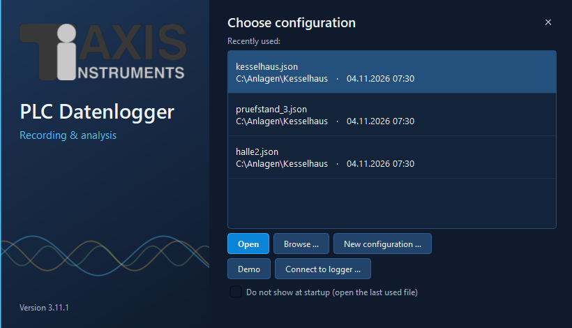
Start screen of the configuration program: choose or create a configuration.
Recently used: the configurations opened last, with folder and modification date. Double-click or Open (Enter key) starts with the selected file.
Browse …: choose any configuration file.
New configuration …: in the logger you are asked for a file name, an empty configuration is created and the configuration program is opened as well; in the configuration program a new, not yet saved configuration begins.
Demo (logger only): start with simulated values.
Do not show at startup: in future start immediately with the last used file. To switch it on again: in the logger File → Show start screen at program start.
After the choice, the start screen shows the loading progress until the main window is
ready. If a configuration file is passed on the command line (e.g.
PLCLogger.exe plant.json), there is no choice. The window can be moved with the
mouse; Esc or ✕ quits.
Quick start
Start
plc_config.py.In the tab Project & controllers enter a project name and the controller(s): Name, choose the Driver, set up the connection with … (IP address and the parameters of the driver), interval.
Take variables from the controller with the selection button of the driver (e.g. Select from variable list…, Select from tag list…, Select from DB source…), or enter the address by hand with Add variable.
Check with Test connection that the values are read correctly.
Save (or Save as… with a file name of your own) and close the configuration program.
Start
plc_logger.pyand press ▶ Start.
Tip
An existing configuration of the S7, TIA or CLX data logger is simply opened with File › Open… (see Importing configurations of the single programs). Without a PLC you can try the program in Demo mode (see Demo mode).
Configuration program (plc_config.py)
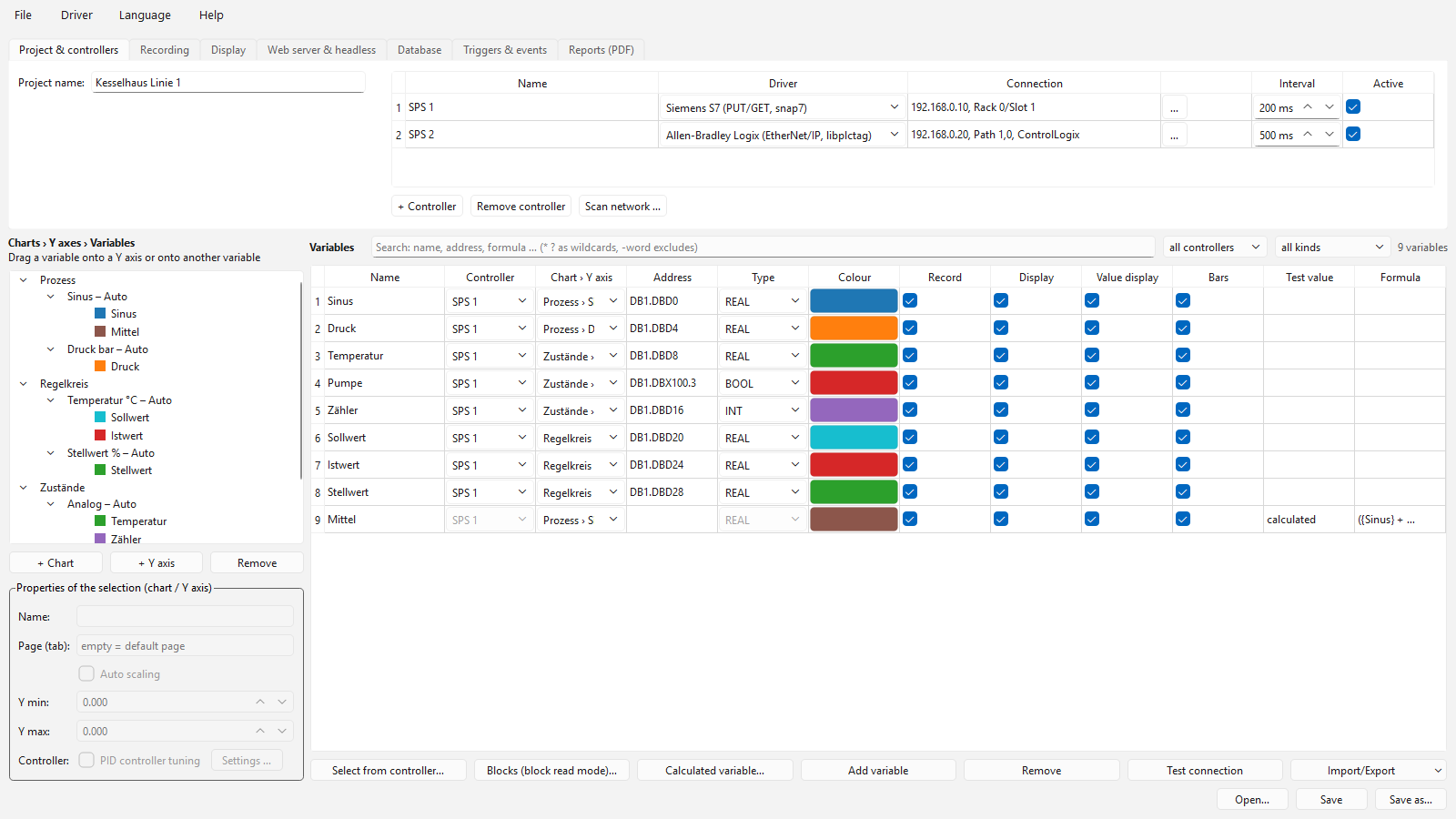
The configuration program: tabs at the top, assignment tree on the left, variable table on the right.
Project, controllers and settings
The upper part of the window is divided into several tabs.
Tab “Project & controllers”

Tab “Project & controllers”.
Field |
Meaning |
|---|---|
Project name |
Freely chosen name of the project. It appears in the window titles, in the web server and in the log. |
Controllers (table) |
One row per controller with the columns:
Change the list with + Controller and Remove controller; when a controller is removed, its variables and blocks move to the first controller. Scan network … finds reachable controllers: in the range (suggestion:
the own network, e.g. |
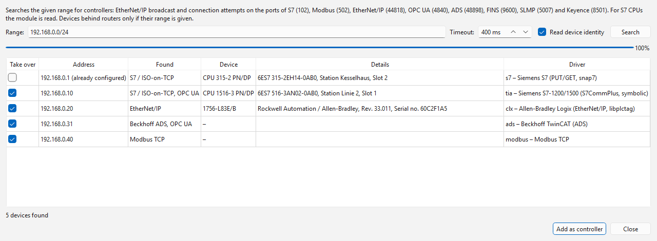
Scan network: controllers found with identity and driver suggestion; the address already configured is not preselected.
Connection settings dialog. The dialog is built from the driver’s parameters (text fields, numbers, choice lists, password fields). Rarely needed parameters are in the Advanced section. At the bottom the dialog shows whether the required library is installed (✓ or ✗ with error message). On OK the driver checks the input (e.g. an empty IP address). The parameters of the built-in drivers are described in the chapter Controllers and drivers.
In the logger, each controller is read by its own thread. The interval applies per controller; a slow or failed controller does not slow down the others. The measurements of all controllers – whatever their driver – are merged into one common CSV file (one column per variable).
Menu “Driver”
Installed drivers … – overview of all loaded drivers with ID, name, required library and its state; below, drivers that could not be loaded (with error message), and the folder for own drivers.
Open folder for own drivers … – creates the folder
treiberin the data folder (if necessary), copies the template_vorlage.pyinto it and opens it in the file manager (see Developing drivers).
Tab “Recording”

Tab “Recording”.
Field |
Meaning |
|---|---|
Write CSV file |
Switches the CSV file on or off (e.g. off if recording only to a database; see Database recording). |
CSV folder |
Target folder for the log files. A relative path refers to the program folder. |
CSV name |
Name of the recording. It is the prefix of the file names and the name of the
archive subfolder (default: |
Max. records per file |
Upper limit for the number of records (rows) per CSV file. |
Archive folder |
Base folder of the archive (default: |
Archive when closing |
If ticked (default), the current, not yet full CSV file is also zipped and archived when the logger is closed. |
Delete after, Use at most |
Clean-up of old recordings of this logger (CSV files and archive ZIPs): files whose last change is more than n days ago are deleted; if all together take up more than n MB, the oldest are deleted until the limit is met. never/ unlimited (0) = off. See Cleaning up old recordings. |
Recording |
Continuous (default) or By trigger with pre- and post-trigger time: then data is only saved while the start condition is met (see Recording by trigger (pre- and post-trigger)). |
Start condition |
Condition as for triggers, e.g. |
Pre-trigger, post-trigger, max. |
Seconds before the trigger (ring buffer), after the end of the condition, and the maximum duration of a capture (unlimited = 0). |
Tab “Display”

Tab “Display”.
Field |
Meaning |
|---|---|
Display window (online) |
Width of the visible time window in online mode, in seconds. |
Default page layout |
Layout at start: Stacked, Side by side or Tabs. |
Charts on one page |
Automatic (like the default layout), Stacked, Side by side or Grid. |
Grid columns |
Number of columns for Grid; automatic derives it from the number of charts. |
Show bars for current values |
Switches the narrow bars next to the charts on by default. |
Bar width |
Width of a bar in pixels (4 … 40, default 14). |
Logo |
Image file, e.g. the company logo. It appears in the logger at the top right of
the menu bar (28 pixels high), on the web pages (charts, process view, login) and
in the header of PDF reports and IO check protocols. PNG and JPG work everywhere,
SVG only in the logger and on the web pages. A relative path refers to the
program folder. Empty = supplied manufacturer logo ( |
Customer logo |
Second logo (e.g. of the customer or plant), shown in the same places to the left of the logo, in the PDF at the top left. Empty = no customer logo. |
Program icon |
Icon for windows and taskbar of the logger and the event log (PNG, ICO or SVG).
Without an entry the program’s own icon is used (folder |
Tab “Database”

Tab “Database”.
Choice and access data of a database that is recorded to in addition to or instead of the CSV file (SQLite, MariaDB/MySQL, TimescaleDB/PostgreSQL, QuestDB, InfluxDB 3, VictoriaMetrics, Prometheus), with the button Test database. Details in the chapter Database recording.
Tab “Triggers & events”

Tab “Triggers & events”.
Shows the number of triggers defined. Edit triggers … opens the trigger editor, Show event log … the event viewer, and Event file sets where the event log is stored (empty = next to the CSV file). Details in the chapter Triggers and event log.
Tab “Reports (PDF)”
Field |
Meaning |
|---|---|
Create PDF report automatically |
At the end of each period the logger writes a report (also in headless operation); a partial report is created when stopping. |
Period |
Shift, Day, Week (from Monday) or Month. |
Shift starts |
Times separated by commas, e.g. |
Day start |
Time at which day, week and month begin (e.g. |
Folder |
Target folder (default |
Details in the chapter PDF reports.
Tab “Web server & headless”

Tab “Web server & headless”.
Field |
Meaning |
|---|---|
Start web server |
Starts a web server together with the logger (see Web server (charts in the browser)). |
Address (host) / port |
|
Access code |
Optional. If a code is set, it must be given when opening the page with
|
Browser refresh |
How often the browser page fetches new data (200 to 60000 ms). |
Headless mode |
The logger starts without user interface and only records (see Headless operation (recording only)). |
Headless loggers |
Running loggers … shows the running headless loggers and stops them cleanly on request; next to it is the number of running loggers. |
HTTPS (encrypted) |
Encrypted connection. Without a certificate of your own, the program creates a
self-signed one once (folder |
Certificate / key (PEM) |
Optionally your own certificate and key (e.g. from the company CA). |
Login |
Users … creates users with password (only a hash is stored). Without users no login is needed. See HTTPS and login. |
Structure: charts, Y axes and variables
The display is structured hierarchically:
Chart
├── Y axis 1 (left)
│   ├── Variable A
│   └── Variable B
└── Y axis 2 (right)
    └── Variable C
Each chart appears in the logger as its own movable window.
Each chart has at least one Y axis. The first axis is on the left, all others on the right. Each axis scales independently.
Each variable belongs to exactly one Y axis of one chart.
The tree on the left shows this structure. Below it are the buttons:
Button |
Effect |
|---|---|
+ Chart |
Creates a new chart with one Y axis. |
+ Y axis |
Adds another Y axis to the selected chart (or the chart of the selection). |
Remove |
Removes the selected chart, Y axis or variable. Affected variables move to the first axis or the first chart. The last chart and the last axis of a chart cannot be removed. |
Properties of chart and Y axis
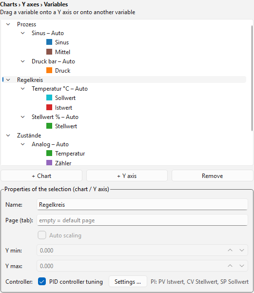
Properties of the selected chart or Y axis.
Select a chart or a Y axis in the tree. In the Properties area below you can change:
Field |
Meaning |
|---|---|
Name |
Name of the chart or Y axis (shown as title or axis label). |
Page (tab) |
Charts only. Charts with the same page name are shown together on one page
(tab or dock), e.g. |
Controller |
Charts only. Tick PID controller tuning and Settings …: define setpoint, process value and controller output for calculating the controller parameters in the logger (see PID controller tuning). |
Auto scaling |
Y axes only. Active: the axis adapts automatically to the visible data. Inactive: the fixed limits Y min and Y max apply. |
Y min / Y max |
Fixed axis limits. Y max must be greater than Y min. |
Creating variables
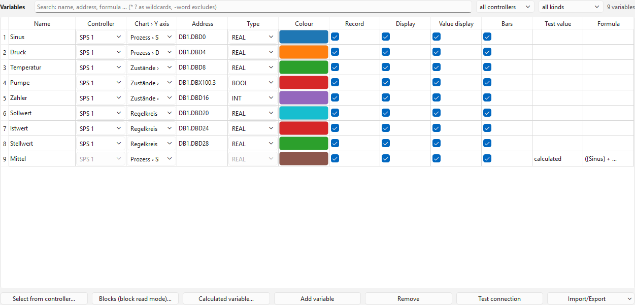
The variable table with controller, address, type, colour and formula.
Each row of the variable table describes one value of a controller:
Column |
Meaning |
|---|---|
Name |
Unique name (also used as CSV column header). The character |
Controller |
Controller the variable is read from (choice from the controller table). It determines the driver and thus the address notation and the possible types. |
Chart › Y axis |
Assignment of the variable (choice list or drag & drop, see below). |
Address |
Address in the driver’s notation, e.g. |
Type |
Data type, choice of the types the driver can read (e.g. |
Colour |
Line colour; a click opens the colour picker. |
Record |
Active (default): the variable is read from the controller and stored (CSV file, database, report). Off: the variable stays in the configuration with all its settings but is not read – this way variables can be prepared and added to or removed from the recording as needed. Formulas, triggers and PID tuning cannot use variables that are not recorded (message when saving). |
Display |
Active (default): the variable appears in the charts and in the value/ruler table (logger, web server, report, Grafana dashboard). Off: the variable is recorded but not displayed. Only recorded variables can be displayed. |
Value display |
Active: the variable appears in the logger’s value/ruler table. |
Bars |
Active: a narrow bar is shown for the variable next to the chart. |
Test value |
Result of Test connection. |
Formula |
Calculated variables only: the formula (double-click opens the editor). |
Searching and filtering variables
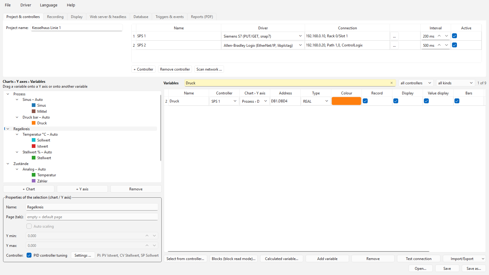
Search field and filters above the variable table.
Above the variable table there are a search field and two choice lists
(Ctrl+F jumps to the search field):
Search text – searches name, address, formula, assignment (chart › Y axis), type and controller; case does not matter. Several words must all match (
temp db10),*and?are wildcards (DB?.DBD*), a word with a leading-excludes (temp -setpoint).Controller – only variables of one controller (calculated variables stay visible).
Kind – read only, computed only, without address (incomplete rows), not recorded or not displayed.
In the variable tree on the left, variables that are not recorded or not displayed are shown in grey with the note (not recorded) or (not displayed).
On the right you see how many variables are currently shown (12 of 340); the search field has a yellow background while a filter is active. Hidden variables stay in the configuration and are saved as well. Remove deletes only selected, visible rows. A newly created variable that does not match the filter resets the filter.
Assignment by drag & drop
Variables can be moved in the tree with the mouse:
Drop onto a Y axis: the variable then belongs to this axis.
Drop onto another variable: the variable takes over the Y axis (and thus the chart) of the target variable.
Drop onto a chart: the variable is assigned to the first Y axis of this chart.
The choice list Chart › Y axis in the table and the tree are always in sync.
Calculated variables (formulas)
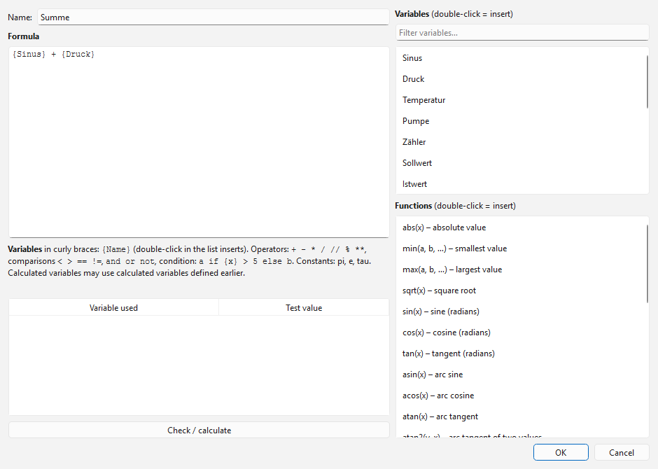
The editor for calculated variables.
Besides the variables read from the PLC you can create calculated variables whose values the logger computes from other variables at every measurement. They appear like normal variables in charts, bars, legend, value table and in the CSV file.
Calculated variable… opens the editor:
Name of the new variable.
Formula in the text field. Variables are written in curly braces, e.g.
({Temp_Vorlauf} + {Temp_Ruecklauf}) / 2. A double-click in the variable list inserts the name, a double-click in the function list the function.Check / calculate: the editor checks the formula (syntax, known variables) and calculates it with freely entered test values. The result appears directly below.
The new variable is assigned to the selected chart or Y axis (changeable like any variable). Double-clicking the Formula column opens the editor again.
Allowed are:
Element |
Example / meaning |
|---|---|
Arithmetic operators |
|
Comparisons, logic |
|
Condition |
|
Constants |
|
Mathematics |
|
Time functions |
|
Examples:
{Prozess.Temperatur} * 1.8 + 32               conversion °C to °F
{Druck_Ein} - {Druck_Aus}                     differential pressure
avg({Durchfluss}, 20)                         smoothed flow
integ({Durchfluss}) / 3600                    total quantity (flow in 1/h)
clamp({Fuellstand}, 0, 100)                   limited to 0 … 100
Notes:
If a value cannot be computed (division by 0, missing measurement, invalid range such as
sqrtof a negative number), the result is no value (empty CSV field, gap in the curve).A calculated variable may only use variables that are further up in the table (real variables always, calculated ones only if defined earlier). This is checked when saving.
If a variable is renamed, formulas using it must be adapted. The name in the formula must match exactly.
For security reasons no arbitrary program code is executed, only the elements listed above.
ddt,integandavgkeep their state during the recording and start anew with every ▶ Start.Calculated variables are not read from the PLC and are missing in Test connection.
Block read mode
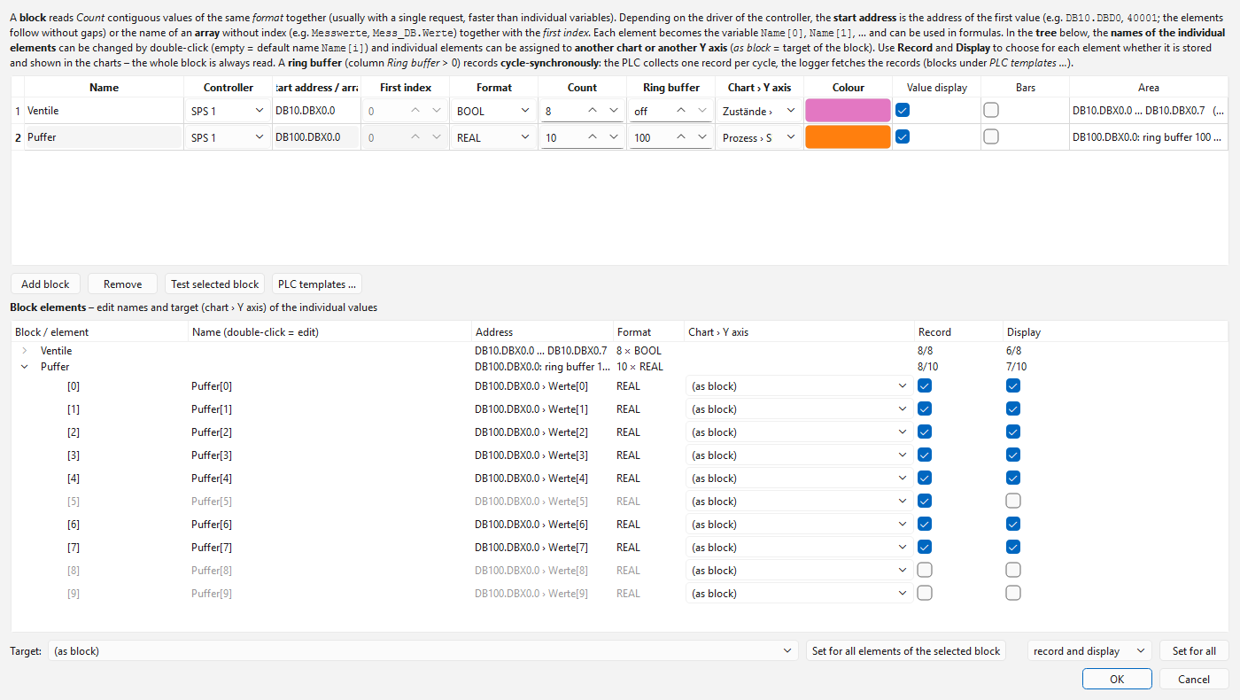
The block editor with block table and element tree (name and target per element).
Many values of the same kind that lie one after another in the controller are read by the block read mode with as few as one request; the values are then assigned individually. What a block is depends on the driver:
Driver |
Block |
|---|---|
|
Start address (e.g. |
|
Array without index (e.g. |
|
Array tag without index (e.g. |
|
Start address (e.g. |
|
like |
|
Array node / array name (without index) + first index + count; read in one request. |
|
Start device / address (e.g. |
|
First element of an N, F, L or B file (e.g. |
|
Start address (e.g. |
Blocks (block read mode)… opens the editor. Each row is a block with the following data:
Field |
Meaning |
|---|---|
Name |
Name of the block. Each element becomes the variable |
Controller |
Controller the block is read from (determines the driver). |
Start address / array |
See the table above; the tooltip shows the driver’s notation. |
First index |
Only for drivers with arrays ( |
Format |
Data type of the elements (choice of the driver). |
Count |
Number of values (1 to 1000). |
Ring buffer |
Number of records of a ring buffer (see Ring buffer); off = normal block.
Drivers |
Chart › Y axis |
Assignment of all elements of the block (single elements can be assigned differently in the tree, see below). |
Colour |
The first element gets this colour, the others differ in hue. |
Value display / bars |
Apply to all elements of the block (bars are off by default). |
Range |
Computed display, e.g. |
Example (clx): array tag Messwerte (REAL[100]), first index 10, count 20
reads Messwerte[10] to Messwerte[29] with one request and creates the
variables Block[0] to Block[19]. Example (s7): start address DB5.DBD0,
format REAL, count 20 reads bytes 0 to 79 of DB 5.
With tia, clx, opcua, ads and s7 (from the DB source), arrays can also be
taken over as a block directly in the selection dialog (select the array, Selected array
as block… or Array as block …, or double-click).
Test selected block reads the block once from the controller and shows the first values and the read time.
Notes:
The block elements are normal variables: they appear in charts, legend, value table, bars and CSV file and can be used in formulas, e.g.
{Messwerte[3]} - {Messwerte[4]}.Record and display per element: In the tree of the block editor every element has the check boxes Record and Display. Elements that are not recorded are not stored (CSV file, database, report); recorded elements without Display do not appear in the charts and the value table. The block is always read completely – elements that are not recorded are therefore still available to formulas and triggers. The displayed elements are distributed over the charts as usual. Below the tree, Set for all sets record and display, record only or do not record for all elements of the selected block. The block row in the tree shows how many elements are recorded and displayed; in the configuration file the exceptions are stored under
nicht_aufzeichnenandnicht_anzeigen(list of element indices).Renaming elements: In the lower part of the block editor a tree shows all blocks with their elements. Double-click the Name column to give an element a name of its own, e.g.
Supply pressureinstead ofMesswerte[1]. An empty name restores the default name. The names must be unique and must not contain; { }. In the configuration file they are stored underelementnamenof the block.Elements in different charts: In the tree of the block editor every element has a choice list Chart › Y axis in the last column. (like block) uses the target of the block, every other entry shows this element in another chart or on another Y axis. Set for all elements of the selected block applies the chosen target to all elements. In the configuration file different targets are stored under
elementziele(index: [chart, axis]).In the variable tree of the configuration each block appears as one row (
▦ Block …) under its Y axis. Remove deletes the selected block.The range must exist completely in the controller (array large enough, DB long enough, registers present), otherwise reading the block fails; the other variables are still read.
Many elements mean many curves: split large blocks over several charts or Y axes or switch off Display or value display for individual elements.
Ring buffer (cycle-synchronous recording)
Normally the logger polls the controller at the configured read interval. How long a request takes varies with the network and the load of the controller; cycles in between are missing, and the time stamp is the time on the PC. For cycle-synchronous, gap-free recording – e.g. every 10 or 50 ms – the controller collects the values itself: a small block writes one record (number, time, values) per cycle or cyclic interrupt into a ring buffer. The logger fetches the new records at the read interval (e.g. every 250 ms) and turns each record into a row of its own with the time stamp of the controller. The sampling rate thus depends only on the controller, not on the network.
Possible with the drivers s7 (S7-300/400, S7-1200/1500 with PUT/GET), tia
(S7-1200/1500 without PUT/GET) and clx (ControlLogix, CompactLogix).
1. Load the block into the controller. The button PLC templates … in the block
editor opens the folder vorlagen with ready-made blocks:
File |
Controller |
Driver |
|---|---|---|
|
S7-300/400 (SCL source for STEP 7 V5.x) |
|
|
S7-300/400 as function block with 20 inputs: the buffer is in the instance DB
(several instances = several ring buffers). Start address |
|
|
S7-1200/1500 (SCL source for TIA Portal: External source files) |
|
|
S7-1200/1500 as function block with 20 inputs: the buffer is in the instance DB
|
|
|
ControlLogix/CompactLogix (Structured Text, data types described) |
|
The templates write 10 values of type REAL into a buffer with 100 records; both numbers can be adjusted (notes at the top of each file). Call the block where the values arise regularly: in a cyclic interrupt (S7-300/400: OB35, S7-1200/1500: Cyclic interrupt OB30, Logix: periodic task) with e.g. 10 ms or 50 ms.
2. Create the ring buffer in the block editor. A block becomes a ring buffer as soon as the column Ring buffer contains the number of records (off = normal block):
Field |
Ring buffer |
|---|---|
Start address |
|
Format |
Data type of the values: |
Count |
Values per record (as in the controller). |
Ring buffer |
Records in the buffer (as in the controller). |
As with blocks, the elements are called Name[0], Name[1] … and can be renamed and
assigned to other charts in the tree. Test selected block fetches the buffer once and
shows the counter, the number of records, their mean interval and the latest values.
3. Read interval and buffer size. The Interval of the controller (table of controllers) is the read interval here: it only determines how often the buffer is fetched. The buffer must hold the records of at least three read intervals: records ≥ 3 × read interval ÷ cycle time. Example: 10 ms cyclic interrupt and 250 ms read interval → at least 75 records (the templates have 100); 50 ms and 500 ms → at least 30.
Buffer layout (S7 with absolute address: non-optimized DB, even start address;
tia with a name and Logix: exactly these names; with tia the arrays may also
start at 1):
Zaehler          DINT     number of records written so far (1, 2, 3 …)
Daten[0..N-1]             N records; record number n is stored in Daten[n MOD N]
  Seq            DINT     number of the record (= Zaehler when written)
  Zeit           DINT     time in ms (see below)
  Werte[0..M-1]           M values in the chosen format
The controller writes in this order: values, time, Seq, finally the counter. The logger reads the counter, then the new records and the counter once more; a record only counts if Seq has the expected number and it could not have been overwritten during reading.
Time: S7-300/400 TIME_TCK (ms since the CPU restart), S7-1200/1500 and Logix ms
since midnight from the controller’s clock. The logger removes overflows (midnight, 2³¹)
and attaches the time to the PC clock: the latest record of the first fetch gets the
current time, all others their distance to it according to the controller. The intervals
between rows are thus exactly those of the controller; the absolute time is as accurate
as the PC clock (a deviating controller clock is followed slowly).
Notes:
Lost records (buffer too small, connection interrupted for a long time) are reported in the status line: “Ring buffer …: n records lost”. After a short interruption the records are fetched from the buffer as long as it still contains them.
A restart of the controller resets the counter; the logger detects this and starts again.
Because the records only arrive when they are fetched, charts and value table show all values delayed by about two read intervals when ring buffers are used (the rows are sorted by their time). CSV file and database contain every record with its time.
Normal variables of the same or other controllers are read as usual; in the rows of a ring buffer they keep their last value.
Formulas, triggers, reports and triggered recording see every record – a trigger thus also fires on a pulse of just one cycle.
In demo mode, ring buffer elements deliver simulated values like normal variables.
Selecting variables from the controller
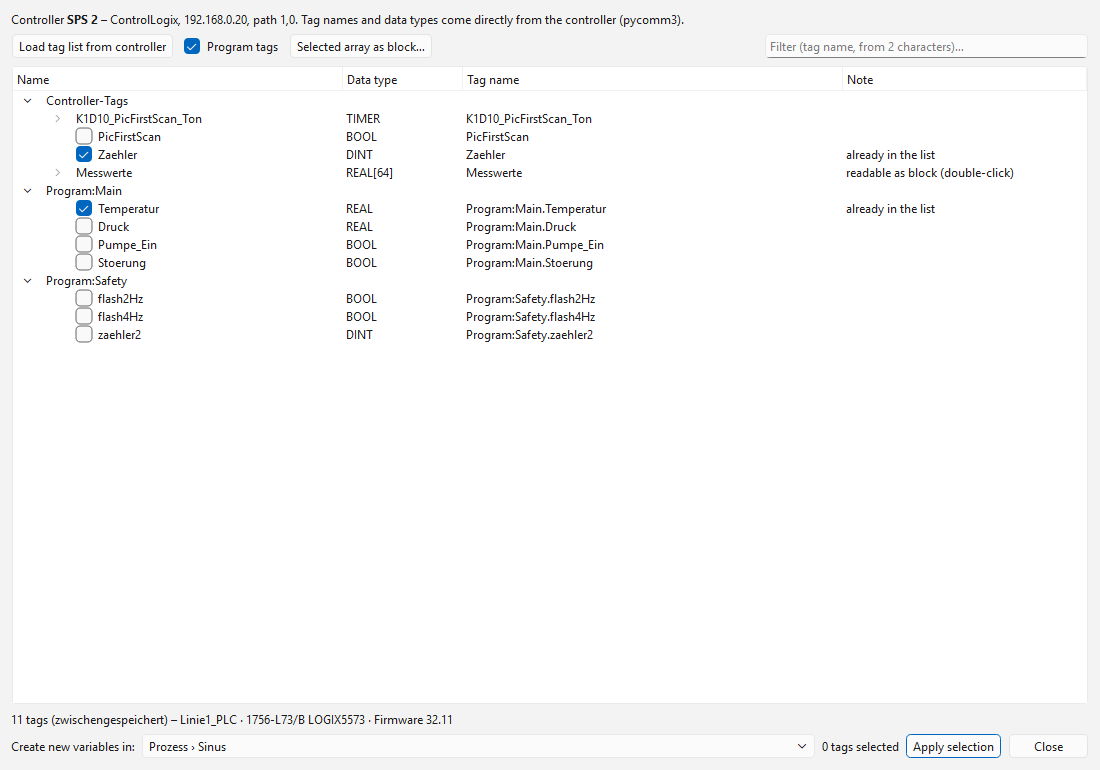
Example: tag list of a ControlLogix (driver clx); tags already created are ticked.
The button above the variable table has a different name depending on the driver of the selected controller and opens its selection dialog (with several controllers you are asked first which one):
Driver |
Button |
Source of the variables |
|---|---|---|
|
Select from variable list… |
Variable list directly from the CPU (all data blocks, memory, inputs and outputs with structure and type, including optimized blocks). |
|
Select from tag list… |
Tag list directly from the controller (pycomm3): controller and program tags, UDTs, arrays. |
|
Select from DB source… |
Exported DB sources from TIA Portal/STEP 7 (the PLC delivers no names via PUT/GET); comparison of the DB sizes with the PLC, arrays as block. |
|
Select from OPC UA server… |
Address space of the server (folders, variables with data type, arrays as block). |
|
Choose from TwinCAT… |
Symbol table of the TwinCAT controller (tree by name parts, type, comment, arrays as block). |
other drivers |
– |
Modbus, MELSEC, Omron, KEYENCE, TOYOPUC, LOGO!, MicroLogix and S5 deliver no names; enter the addresses by hand as per program or device manual. |
General procedure:
Load. When opened for the first time, the list is loaded from the controller (
tia,clx) or the DB sources are imported (s7, Import DB source…). Loaded lists are cached per controller in the foldertaglistenof the data folder and are shown immediately the next time, even without a connection. The paths of the S7 DB sources are stored in the configuration.Search. Structures and arrays can be expanded; the filter field searches by name.
Select. Tick readable values. Variables already created are ticked and greyed out. Types that cannot be recorded (e.g.
STRING) are shown in grey.Arrays as block (
tia,clx,opcua,ads,s7): select the array, Selected array as block… (s7: Array as block …) or double-click, set first index and count. Withs7this applies to one-dimensional arrays of numbers or BOOL; the start address is calculated from the DB source.Take over. Under Create new variables in choose the chart or Y axis and press Take over selection. Address and type come from the controller or source.
Check. Check the values read with Test connection.
Details about the dialogs are given for each driver in the chapter Controllers and drivers.
Testing the connection
Test connection connects to each controller in turn (via its driver), reads its variables once and enters the result in the Test value column. Errors of single variables are shown there in plain text (e.g. address does not exist, wrong type, access denied, Modbus exception “illegal address”); if a controller cannot be reached, a message box reports it with name and connection.
When saving, the driver of each controller checks the addresses formally (notation,
suitable type, e.g. BOOL for coils). Whether an address actually exists in the
controller is only shown by the connection test.
Saving and loading
The File menu of the configuration program contains:
New – empty configuration with one controller; the file name is asked for when saving for the first time.
Open… (
Ctrl+O) – loads a configuration file (JSON) with any name, including configurations of the S7, TIA and CLX data loggers (see Importing configurations of the single programs).Save (
Ctrl+S) and Save as… (Ctrl+Shift+S) – write to the current or a new file (the extension is always.json). Before saving it is checked that controller and variable names are unique and not empty, the connection parameters and addresses are valid for the respective driver, the formulas are correct and, for fixed Y axes, Y max is greater than Y min.Convert INI file … – convert older INI configurations once to JSON (see Converting older INI files).
Start logger with this configuration (
Ctrl+R) – saves and starts the logger with this file.Start IO check with this configuration – saves and starts the IO check with the controllers of this file (separate program).
Show/stop headless loggers … – show running headless loggers and stop them cleanly (see Headless operation (recording only)).
Export Grafana dashboard … – dashboard with the layout of the logger as a JSON file for Grafana (see Database recording).
The window title shows project name and file name. The last used file is remembered
(file plc_last.txt); the logger and the configuration program open it again at the
next start without parameters.
Note
The logger reads the configuration at every start. Changes therefore only take effect after pressing ▶ Start again.
Importing and exporting variables
The Import/Export button below the variable table exchanges the variable list with
an Excel (.xlsx) or CSV file – useful for editing long lists in Excel or for
taking over an address list of the controller. ODS files (LibreOffice/OpenOffice
Calc, .ods) can be read as well.
Export variables (CSV/Excel) … writes all variables of the table (without block elements, see Block read mode) with the columns
Name,Steuerung,Diagramm,Y-Achse,Adresse,Typ,Farbe,Aufzeichnen,Anzeigen,Werteanzeige,BalkenandFormel. The column names are always German, so files can be exchanged between languages.Import variables (CSV/Excel/ODS) … reads such a file. The first row contains the column names; only
Nameis mandatory, order and case do not matter. CSV files may use semicolon, comma or tab as separator.
When importing:
If variables already exist, the program asks whether they should be replaced or the new ones appended. When appending, variables with an existing name are skipped.
Steuerungis the name of a controller from the controller table; empty or unknown = first controller (unknown names are reported).DiagrammandY-Achseare names; missing charts and axes are created, empty = first chart or first axis.Typempty = default type of the driver;Farbeas#rrggbb, empty = colour from the palette.Aufzeichnen,Anzeigen,WerteanzeigeandBalken:ja/nein(alsoyes/no,1/0,x); empty = yes.If
Formelis filled, a calculated variable is created (AdresseandTypare then ignored).
As with manual input, addresses and formulas are only checked when saving.
Structure of the configuration file (JSON)
The configuration is saved as a JSON file (UTF-8, indented) and can also be edited by hand if required – with any text editor, preferably one that checks JSON (e.g. Notepad++, Visual Studio Code). The keys are German. Example:
{
  "format": "PLC Datenlogger Konfiguration",
  "version": 1,
  "einstellungen": {
    "projekt": "Prüfstand 3",
    "csv_ordner": "logs",
    "csv_name": "log",
    "max_records": 100000,
    "archiv_ordner": "archiv",
    "fenster_s": 60,
    "anordnung": "untereinander",
    "balken": true,
    "archiv_beenden": true,
    "seite_anordnung": "raster",
    "raster_spalten": 2,
    "web_aktiv": true,
    "web_host": "0.0.0.0",
    "web_port": 8080,
    "web_intervall_ms": 1000,
    "headless": false,
    "treiberdaten": {
      "s7": {
        "symbolquellen": "C:/Projekt/Mess_DB.db"
      }
    }
  },
  "steuerungen": [
    {
      "name": "Presse",
      "treiber": "tia",
      "intervall_ms": 100,
      "aktiv": true,
      "ip": "192.168.0.1",
      "port": 102,
      "tls": "auto",
      "passwort": "",
      "rolle": "hmi",
      "tags_je_anfrage": 50
    },
    {
      "name": "Altanlage",
      "treiber": "s7",
      "intervall_ms": 500,
      "aktiv": true,
      "ip": "192.168.0.20",
      "rack": 0,
      "slot": 2
    },
    {
      "name": "Kessel",
      "treiber": "clx",
      "intervall_ms": 200,
      "aktiv": true,
      "ip": "192.168.1.10",
      "pfad": "1,0",
      "cpu": "controllogix",
      "timeout_ms": 2000
    },
    {
      "name": "Zaehler",
      "treiber": "modbus",
      "intervall_ms": 1000,
      "aktiv": true,
      "ip": "192.168.0.50",
      "port": 502,
      "unit": 1,
      "wortfolge": "CDAB",
      "max_register": 120,
      "luecke": 8,
      "timeout_ms": 2000
    }
  ],
  "diagramme": [
    {
      "name": "Prozess",
      "seite": "Prozess",
      "achsen": [
        {
          "name": "Temperatur",
          "auto": true,
          "y_min": 0.0,
          "y_max": 100.0
        },
        {
          "name": "Leistung",
          "auto": false,
          "y_min": 0.0,
          "y_max": 50.0
        }
      ]
    }
  ],
  "variablen": [
    {
      "name": "Kraft",
      "adresse": "Presse_DB.Kraft",
      "typ": "REAL",
      "farbe": "#d62728",
      "wert_anzeigen": true,
      "diagramm": 1,
      "achse": 1,
      "balken": true,
      "formel": "",
      "steuerung": 1
    },
    {
      "name": "Temp_Alt",
      "adresse": "DB10.DBD4",
      "typ": "REAL",
      "steuerung": 2
    },
    {
      "name": "Temperatur_Kessel",
      "adresse": "Program:Kessel.Temperatur",
      "typ": "REAL",
      "steuerung": 3
    },
    {
      "name": "Wirkleistung",
      "adresse": "30013",
      "typ": "REAL",
      "steuerung": 4
    }
  ],
  "bloecke": [
    {
      "name": "Messwerte",
      "adresse": "Messwerte",
      "start": 0,
      "typ": "REAL",
      "anzahl": 20,
      "diagramm": 1,
      "achse": 1,
      "farbe": "#1f77b4",
      "wert_anzeigen": true,
      "balken": false,
      "steuerung": 3,
      "elementziele": {
        "3": [
          1,
          2
        ]
      }
    }
  ]
}
Structure:
Key |
Content |
|---|---|
|
File identifier and version of the structure (currently 1). |
|
Settings: project, recording (CSV, archive, database, trigger recording, reports), display, web server, headless. |
|
List of controllers (order = number referred to by |
|
List of charts, per chart the list |
|
Normal and calculated variables ( |
|
Blocks of the block read mode; |
|
Triggers of the event log. |
Numbers and booleans are stored with their type (200, 1.5, true/false).
Missing keys get their default value when loading, unknown ones are ignored. If the
file is not valid JSON (e.g. a forgotten comma), the program reports the line of the
error.
Explanations:
treiberis the ID of the driver; the other keys of an entry insteuerungen(exceptname,intervall_ms,aktiv) are its connection parameters (see Controllers and drivers). Unknown keys are ignored, missing ones get the driver’s default value.adresseis the address in the notation of the controller’s driver. For blocks,adresseis the start address or the array name andstartthe first index (drivers with arrays only).treiberdatencontains driver-specific data as an object (e.g. the paths of the S7 DB sources).diagramm,achseandsteuerungare numbers starting at 1.seite_anordnungis empty (automatic),untereinander(stacked),nebeneinander(side by side) orraster(grid);raster_spalten: 0chooses the number of columns automatically.The variables of a block (
Messwerte[0]…) are created when loading and are not listed undervariablenin the file.The TIA password is stored in plain text in the file.
Converting older INI files
Earlier versions stored the configuration as an INI file. These files are no longer opened directly but converted once into a JSON file; the INI file itself remains unchanged:
Configuration program › File › Convert INI file … – choose one or more INI files; a
.jsonfile with the same name is created next to each. For a single file the result is opened immediately.If an INI file is chosen in the configuration program (Open, start screen), it offers the conversion directly.
For many files at once (Python sources):
python tools/ini2json.py plant1.ini plant2.ini        # -> plant1.json, plant2.json
python tools/ini2json.py old.ini -o new.json -f       # other name, overwrite
When started with an INI file, the logger reports that it has to be converted. If an
INI file was opened last and the converted .json file already exists next to it,
that file is used automatically. All contents – including triggers, PID settings and
blocks – are taken over.
Controllers and drivers
Each controller of the configuration has exactly one driver. It defines which connection parameters exist, how variables are addressed, which data types can be read, what blocks look like and whether there is a selection dialog. Any drivers can be mixed in one configuration.
How well is each driver tested? Automatic tests run on every upload; where a
third-party, widely used counterpart exists, they test the driver against its simulator.
So far s7 and clx have been tried with real controllers, tia with the simulated
CPU of S7-PLCSIM Advanced:
Driver |
Tested |
|---|---|
|
With a controller (S7-300/400, also ring buffer; Windows and Raspberry Pi with Ubuntu 24.04); automatically against the S7 server of python-snap7 (single values, bits, blocks, ring buffer). |
|
With a controller (normal reading and blocks; Windows and Raspberry Pi with Ubuntu 24.04); the ring buffer only against a simulated libplctag. |
|
With S7-PLCSIM Advanced (simulated S7-1500) tried successfully: without PUT/GET, with TLS, variable list from the CPU, reading from two optimized DBs, ring buffer by its name, different access levels of the CPU without password (reading or message). Not yet tried: login with password, real CPU. Automatically: ring buffer with absolute address against the S7CommPlus emulator of s7commplus, with a name (optimized) against a simulated controller. |
|
Automatically against the Modbus TCP server of pymodbus (all four tables, bits, REAL/DINT, word order). |
|
Over the network against the logger’s own OPC UA server (Raspberry Pi as server, PC as client): selection dialog, cyclic read, subscription, reconnect after a server failure, Basic256Sha256 (sign and encrypt) with login. Not yet tried: array as block, the server of a real PLC. Automatically against an OPC UA server of asyncua (numbers, BOOL, array as block). |
|
Not yet tried with a controller or a simulator. Experience reports and error reports (e.g. via GitHub) are welcome. |
Driver s7 – Siemens S7 (PUT/GET, snap7)
For S7-300/400 and S7-1200/1500 via classic S7 communication with absolute
addresses. Library: python-snap7.
Parameter |
Meaning |
|---|---|
IP address |
Address of the CPU or CP. |
Rack |
Rack, almost always |
Slot |
Slot of the CPU: S7-300 |
Preparation: On S7-1200/1500 enable “Permit access with PUT/GET communication from
remote partner” in the CPU properties in TIA Portal. Only data blocks without
“Optimized block access” are read (use the tia driver for optimized blocks). TCP
port 102.
Addresses (German or English mnemonics; the type comes from the Type column, the size letter X/B/W/D in the address is only a writing aid):
Address |
Meaning |
|---|---|
|
Data block 10, byte 4 (bit 2) |
|
Short form: DB number, byte[, bit] |
|
Memory (flags) |
|
Inputs (process image) |
|
Outputs (process image) |
When saving, the address is written uniformly to match the type (e.g. DB10.4 with
type REAL → DB10.DBD4).
Types: BOOL, BYTE, USINT, SINT, CHAR, WORD, UINT,
INT, DWORD, UDINT, DINT, REAL, TIME (ms), LWORD, ULINT,
LINT, LREAL.
Blocks: start address + count, elements without gaps; a block is read with one request. Single variables are read individually – with many variables in one DB a block is considerably faster.
Selection dialog “Select from DB source…”: Via S7 communication the PLC delivers no names and structures. The tree of data blocks (DB › structure › variable) is therefore built from DB sources:
In TIA Portal select the DB (and the UDTs needed), right-click Generate source from blocks; in STEP 7 save the DB as source (
.db/.awl).In the dialog choose Import DB source… (several files possible). If the DB number is missing in the source (TIA), it is asked for.
Optionally Compare with PLC: compares the computed size of each DB with the size in the PLC (✓ or ⚠ – a difference indicates an optimized block or an outdated source).
Tick variables (a tick on a structure/array/DB selects everything in it) and take them over. The name of the variable is the symbol path.
The paths of the sources are stored in the configuration (treiberdaten) and read
again the next time.
Driver tia – Siemens S7-1200/1500 symbolic (S7CommPlus)
Symbolic access like TIA Portal and Siemens HMIs – also to optimized data blocks,
without PUT/GET. Library: s7commplus.
Parameter |
Meaning |
|---|---|
IP address |
Address of the CPU. |
Port |
ISO-on-TCP port, default |
TLS |
Automatic (TLS if the CPU offers it), Off, On (force TLS). Newer firmware (S7-1500 from V3.1, S7-1200 from V4.7, projects from TIA V19) communicates only encrypted. |
Password |
Password of the access level if the CPU protects read access (stored in plain text in the configuration file). |
Role (Advanced) |
HMI (default), Engineering, PG. |
Variables per request (Advanced) |
Maximum number of variables per read request (default 50); larger quantities are split. |
Preparation: usually none. Variables must be “Accessible from HMI/OPC UA/Web API” (default). Each CPU allows only a limited number of HMI connections; the logger uses one per controller. TCP port 102.
Addresses: symbolic names as in TIA Portal:
Mess_DB.Temp                     variable in a data block
Anlage_DB.Motor[2].Drehzahl      structure member in an array
MArea.Start_Merker               memory (PLC tag)
IArea.Taster_1                   input
QArea.Lampe                      output
Types: BOOL, BYTE, WORD, DWORD, LWORD, SINT, INT,
DINT, LINT, USINT, UINT, UDINT, ULINT, REAL, LREAL,
TIME, LTIME, S5TIME, CHAR, WCHAR.
Blocks: array without index + first index (as in TIA, e.g. 1 for
Array[1..100]) + count.
Selection dialog “Select from variable list…”: loads the variable list directly
from the CPU (data blocks, memory, inputs/outputs with structure and type) and caches it
in the folder taglisten.
Warning
s7commplus is an unofficial implementation, not from Siemens. Test new
configurations on a plant that is not safety-relevant first.
Driver logo – Siemens LOGO! (0BA7/0BA8)
For LOGO! 7 (0BA7) and LOGO! 8 (0BA8, 8.FS4, 8.3, 8.4) via S7 communication; library
python-snap7 (as for the s7 driver).
Set up in the LOGO!: In LOGO!Soft Comfort under Tools › Ethernet Connections
(LOGO! 8: Online Settings › Access control) enable HMI access or create a server
connection (S7). The TSAP values of this connection must match the parameters here:
Local TSAP of the LOGO! = TSAP of the LOGO!, Remote TSAP = TSAP of the
logger. LOGO! 8 with HMI access enabled: 02.00 and 01.00 (default).
Parameter |
Meaning |
|---|---|
IP address |
Address of the LOGO!. |
Device |
LOGO! 8 or LOGO! 7 – determines where I, Q, M, AI, AQ, AM are located in the variable memory (VM). |
TSAP of the LOGO! / TSAP of the logger |
As |
Addresses: variable memory directly (V10 or VB10 = byte, VW12 = word,
VD20 = double word, V10.3 = bit) or the LOGO! operands I1 … I24,
Q1 … Q20, M1 … M64, NI, NQ (BOOL) and AI1 … AI8,
AQ, AM1 … AM64, NAI, NAQ (INT). Values in the VM are “big endian” as
with S7. Neighbouring addresses are merged into one request; blocks: start address in
the VM (e.g. VW100), the elements follow without gaps.
Driver clx – Allen-Bradley Logix (EtherNet/IP)
For ControlLogix, CompactLogix and Micro800. Reading is done with libplctag
(plctag.dll / libplctag.so); all tags of a controller are triggered at the same
time in each cycle and combined into common CIP requests. The tag list is provided by
pycomm3.
Parameter |
Meaning |
|---|---|
IP address |
Address of the Ethernet module (e.g. 1756-EN2T) or of the CPU with built-in Ethernet. |
CIP path |
Route to the CPU, |
Controller type |
ControlLogix, CompactLogix or Micro800. |
Timeout (Advanced) |
Waiting time per read cycle (default 2000 ms). |
Preparation: External Access of the tags Read/Write or Read Only. TCP port 44818.
Addresses: tag names as in Studio 5000 or Connected Components Workbench:
Temp_Kessel (controller tag), Program:Main.Druck (program tag),
Anlage.Motor[2].Drehzahl, Status.3 (bit 3 of an integer, type BOOL).
Types: BOOL, SINT, INT, DINT, LINT, USINT, UINT,
UDINT, ULINT, REAL, LREAL (read bit strings DWORD/WORD as
UDINT/UINT).
Blocks: array tag without index + first index + count; libplctag splits large ranges itself. BOOL arrays not as block.
Selection dialog “Select from tag list…”: controller tags and (tick Program tags)
the tags of all programs, with UDTs, arrays (at most 500 elements individually) and
filter; cached in the folder taglisten.
Driver pccc – Allen-Bradley MicroLogix / SLC 500 (PCCC)
For the older Allen-Bradley controllers with file addresses (RSLogix 500): MicroLogix
1100/1400, SLC 5/05 and SLC 5/03/04 via an Ethernet bridge module. Library
pycomm3 (SLCDriver, EtherNet/IP with PCCC commands). ControlLogix, CompactLogix and
Micro800 use the clx driver.
Parameter |
Meaning |
|---|---|
IP address |
Address of the controller or Ethernet module. |
CIP path (Advanced) |
Only behind a bridge module, e.g. |
Addresses in RSLogix 500 notation: N7:0 (INT), F8:2 (REAL), L9:0 (DINT,
MicroLogix 1100/1400), B3:2 (word) or B3:0/5 and N7:10/3 (bits, type
BOOL), T4:0.ACC/T4:0.PRE/C5:1.ACC (accumulated/preset values), T4:0.DN
(status bit), I:0/1, O:0/2, S:1/5. Elements of the same N, F, L or B file
that are close together are read with one request; blocks: first element, e.g.
N7:0.
Driver modbus – Modbus TCP
For all devices with Modbus TCP (also Modbus RTU devices behind a TCP gateway). No additional library. Neighbouring addresses are automatically combined into as few requests as possible (functions 1 to 4).
Parameter |
Meaning |
|---|---|
IP address, port |
Address of the device or gateway, default port |
Device address (unit ID) |
Slave/unit ID (default 1); for gateways the address on the serial bus. |
Byte/word order |
Order for values spanning several registers ( |
Registers per request (Advanced) |
Maximum number of registers in one request (1 to 125, default 120). |
Merge gaps up to (Advanced) |
Addresses with a smaller distance are read in the same request (default 8 registers; 0 = only without gaps). |
Timeout (Advanced) |
Time to wait for a response (default 2000 ms). |
Addresses – Modicon notation (counted from 1) or table + offset (from 0):
Modicon |
from 0 |
Area, function |
|---|---|---|
|
|
Holding registers, FC 3 |
|
|
Input registers, FC 4 |
|
|
Coils, FC 1 (type |
|
|
Discrete inputs, FC 2 (type |
|
|
Bit 3 of a register (type |
40001 and HR0 denote the same register. If the device manual says “register
100” without anything else, it usually means HR100 (= 40101) – if in doubt,
check both with Test connection. %MW0 (Schneider) is understood as HR0.
Types: BOOL, INT, UINT, WORD (1 register), DINT, UDINT,
DWORD, REAL (2 registers), LINT, ULINT, LWORD, LREAL (4
registers).
Blocks: start address + count, elements without gaps (for REAL at a distance
of 2 registers).
Errors: If the device responds with a Modbus exception (e.g. illegal address), only the affected request remains without value; the message appears in the status line or as test value.
Driver modbus_rtu – Modbus RTU (serial)
For devices with Modbus RTU on RS-485 or RS-232 (frequency converters, energy meters,
temperature controllers, compact controllers …), connected via a built-in interface or
a USB adapter. Libraries: pymodbus (3.x or 4.x) and pyserial.
Addresses, data types, byte/word order, blocks and merging of neighbouring addresses
are the same as for the modbus driver (40001/HR0,
30001/IR0, 00001/C0, 10001/DI0, 40001.3).
Parameter |
Meaning |
|---|---|
Port |
Windows |
Device address |
Modbus slave address 1–247. |
Baud rate, parity, stop bits |
As per device; usually 19200 baud, even parity, 1 stop bit (or 9600 8N2). |
Byte/word order |
As for the |
Data bits, registers per request, gap, timeout, retries (Advanced) |
Registers per request default 60 (smaller values relieve slow devices), timeout 1000 ms, 1 retry. |
Several devices on one bus: create one controller per device with the same port and its own device address. The controllers share the port automatically; the telegrams go onto the bus one after the other. Baud rate, parity, stop bits and data bits must be the same (otherwise the second controller reports an error). The sampling intervals of all devices together must match the bus speed – at 9600 baud a request with 10 registers takes about 30 ms.
If a device does not respond, only its controller is reported as faulty (LED red); the other devices on the bus are still read.
Driver opcua – OPC UA
For all controllers and servers with OPC UA – e.g. Beckhoff TwinCAT, B&R, Codesys
controllers (Wago, Festo, Schneider, Eaton …), Siemens S7-1500 and WinCC, Omron NX/NJ,
Rockwell via FactoryTalk Linx Gateway, Mitsubishi iQ-R with OPC UA module,
Kepware/KEPServerEX. Library: asyncua.
Parameter |
Meaning |
|---|---|
Endpoint |
e.g. |
Operating mode |
Read cyclically (Read) (default) or Subscription – the server reports only changes (see below). |
Publishing interval, sampling interval (Advanced, subscription only) |
How often the server sends collected changes or checks the values; |
Security |
None, or Basic256Sha256, Aes128Sha256RsaOaep, Aes256Sha256RsaPss each with Sign or Sign and encrypt – whatever the server offers. |
User, password |
Empty = anonymous. The password is stored in plain text in the configuration file. |
Client certificate, private key (Advanced) |
Only with security. Empty = the driver creates a self-signed certificate when
connecting for the first time (folder |
Timeout, nodes per request (Advanced) |
Default 4 s and 500 nodes per read request (some servers allow fewer; then set e.g. 100). |
Trusting the certificate: With security, the server usually has to accept the client certificate as trusted first (TwinCAT, Codesys, S7-1500: choose “Trust” in the server’s certificate store). The first connection attempt is rejected; after trusting it works.
Addresses: the NodeId of the node as shown by the server and the engineering tool:
ns=4;s=|var|CODESYS Control.Application.GVL.Temperatur     Codesys
ns=4;s=MAIN.fTemperatur                                     TwinCAT
ns=3;s="DB_Prozess"."Temperatur"                            S7-1500
ns=2;s=Kanal1.Geraet1.Temperatur                            Kepware
ns=2;i=1001                                                 numeric identifier
The server delivers each value with its own OPC UA data type; the Type column is for display only. Timestamps (DateTime) are recorded as Unix time, texts cannot be recorded.
Blocks: array node (NodeId without index) + first index + count. The section is read with an index range in one request. An array as single variable reports “Array – please read as block”.
Selection dialog “Select from OPC UA server…”: connects to the server and shows the address space starting at Objects; folders are loaded when expanded. Tick readable variables (numbers, BOOL), take over arrays by double-click or Selected array as block …. The filter field searches the nodes already loaded. The name of the new variable is the path of display names.
All nodes of a controller are read in each cycle with as few read requests as possible. An invalid node (e.g. BadNodeIdUnknown) affects only its own variable.
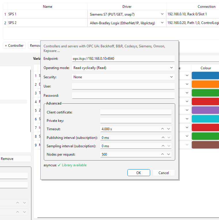
Connection settings of the opcua driver with mode Subscription.
Subscription: Instead of reading all nodes in every cycle, the driver sets up a subscription when connecting; the server then reports only changed values. The logger still records at the interval of the controller (with the last reported value). With many rarely changing values this saves network load and server performance. The initial values are read once; the driver checks the connection every few seconds with a small read request and reconnects if necessary. Arrays (blocks) are subscribed with an index range.
Driver ads – Beckhoff TwinCAT (ADS)
For TwinCAT 2 and 3 via the Beckhoff protocol ADS (AMS/TCP, port 48898) – without an
additional library and without TwinCAT on the logger computer. (Alternatively TwinCAT
also works via the opcua driver if the TF6100 server is licensed.)
Adding a route: The controller answers ADS requests only from computers for which a
route is configured: in the TwinCAT System Manager or XAE under SYSTEM › Routes
(or via the TwinCAT icon on the controller) add a static route with the AMS Net ID of
this computer (parameter Own AMS Net ID, default: IP address + .1.1) and its IP
address. Without a route the driver reports “ADS error 0x7: target machine not found”.
Parameter |
Meaning |
|---|---|
IP address |
Address of the controller. |
AMS Net ID of the controller |
e.g. |
AMS port |
|
Own AMS Net ID, own AMS port (Advanced) |
Must match the route; empty = own IP address + |
Variables per request (Advanced) |
Maximum number of parts of a sum request (TwinCAT: 500). |
Addresses: symbolic as in the PLC project – MAIN.fTemperatur,
GVL.aWerte[3], MAIN.stMotor.nDrehzahl, TwinCAT 2 global .gWert – or
memory/I/O %MW10, %MD4, %MX2.3, %IW0, %QX0.1 or index group:offset
(0x4020:16). Symbol names are resolved once when connecting; afterwards all
variables are read with sum requests (up to 500 per request). After a download to the
controller the driver reconnects and resolves the names again.
Blocks: array name without index (MAIN.aWerte) + first index + count – the
section is read in one piece.
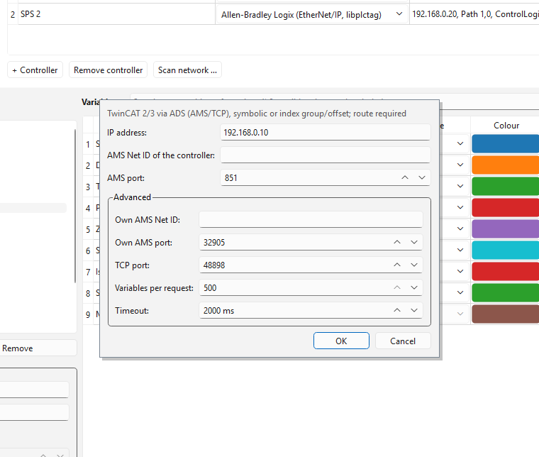
Connection settings of the ads driver (AMS Net ID, ports, advanced).
Selection dialog “Choose from TwinCAT…”: reads the symbol table of the controller
and shows it as a tree (MAIN › Pumpe › fDruck) with type and comment;
filter field, tick variables, take over arrays of numbers as block by double-click.
Driver slmp – Mitsubishi MELSEC (SLMP / MC protocol)
For MELSEC iQ-R, iQ-F (FX5), Q (QnU, QnUDE …) and L with built-in Ethernet or Ethernet module. Protocol SLMP (MC protocol) with 3E frame, binary, via TCP or UDP. No additional library.
Preparation (GX Works): In the Ethernet settings create a connection “SLMP” (iQ-R/iQ-F) or “MC protocol” (Q/L), binary, TCP or UDP, with a port and download it to the controller. The logger only reads.
Parameter |
Meaning |
|---|---|
IP address, port, protocol |
As set in GX Works (e.g. port 5007, TCP). |
Series |
Q/L/iQ-F (standard format) or iQ-R (extended format with 4-byte device numbers). An iQ-R understands both. |
Network no., station, target module (Advanced) |
For the own station |
Words per request, gap, timeout (Advanced) |
Default 960 words (protocol maximum), 16 words, 2000 ms. |
Addresses in MELSEC notation. X, Y, B, W, SB, SW, DX,
DY are hexadecimal, all others decimal:
Address |
Meaning |
|---|---|
|
Word devices (data registers, link registers, file registers …) |
|
Current values of timers, counters, retentive timers |
|
Bit devices (type |
|
Bit 3 of a word (bit |
|
16 bits of a bit device as a word (only from a multiple of 16) |
Types: BOOL, INT, UINT, WORD, DINT, UDINT, DWORD,
REAL, LINT, ULINT, LWORD, LREAL. Values spanning several words
occupy consecutive registers, low word first (as in GX Works).
Blocks: start device + count (e.g. D100, REAL, 10 → D100, D102 …
D118). Independently of this the driver combines neighbouring addresses into as
few requests as possible; bit devices are read word by word (16 bits per word).
Error responses of the controller appear with their code, e.g. SLMP error 0xC056: address out of range; only the respective request is affected.
Driver fins – Omron (FINS)
For Omron CJ1/CJ2, CS1, CP1L/CP1H (Ethernet), CP2E and NJ/NX (with FINS enabled) via FINS/TCP or FINS/UDP, port 9600 – without an additional library.
Parameter |
Meaning |
|---|---|
IP address, port |
Address of the controller or Ethernet unit; port 9600. |
Protocol |
FINS/TCP (recommended; the controller assigns the node numbers) or FINS/UDP. |
Destination/source node, destination/source network (Advanced) |
FINS addresses. |
Words per request (Advanced) |
At most 999 (older CPUs via UDP possibly fewer). |
Addresses in Omron notation (decimal): D100/DM100, W10, H20,
A300, CIO100 (or just 100), extended data memory E0_100 (bank 0 … 24),
timer/counter present values T5, C3; bits with a dot and bit number 00 … 15:
D100.05, CIO0.01, W3.15 (type BOOL). DINT/REAL/LREAL occupy 2 or 4 words,
low word first (as in CX-Programmer). Neighbouring addresses result in one request;
blocks: start address, elements without gaps.
Driver kvhostlink – KEYENCE KV (Host Link)
For KEYENCE KV-8000, KV-7000, KV-5000/5500, KV-3000, KV Nano and KV-X with Ethernet (built-in or KV-EP21V/KV-LE21V). Protocol: Host Link (ASCII) via TCP, port 8501. Nothing needs to be set up in KV STUDIO. No additional library.
Parameter |
Meaning |
|---|---|
IP address, port |
Address of the KV; default port 8501. |
Words per request, gap, timeout (Advanced) |
Default 500 words, 16 words, 2000 ms. |
Addresses in KEYENCE notation:
Address |
Meaning |
|---|---|
|
Word devices |
|
Relays (type |
|
Link relays (hexadecimal, type |
|
Current value of timer or counter (32 bit, type |
|
Bit 3 of a word |
Types as for the slmp driver; values spanning several words: low word first (as
in KV STUDIO). Neighbouring word addresses are read with one RDS command, and so are
neighbouring relays.
Error responses (E0 invalid device number, E1 invalid command …) affect only the
respective request.
Driver toyopuc – JTEKT TOYOPUC (Computer Link)
For JTEKT TOYOPUC PC10G/PC10, PC3J/PC3JG, Nano 10GX and TOYOPUC-Plus with Ethernet. Protocol: Computer Link (binary) via TCP or UDP. No additional library.
Preparation (PCwin): set up a port for Computer Link (TCP passive or UDP) on the Ethernet module or the built-in interface.
Parameter |
Meaning |
|---|---|
IP address, port, protocol |
As set in PCwin. |
Words per request, gap, timeout (Advanced) |
Default 512 words, 16 words, 2000 ms. |
Addresses as in PCwin, numbers hexadecimal:
Address |
Meaning |
|---|---|
|
Registers (data, link, special, current value, file registers) |
|
Relays and contacts (type |
|
16 relays as a word ( |
|
Bit F of a register |
|
Extended registers |
|
Extended relays |
|
Program areas 1–3 (PC3J in 3-program mode, PC10); the upper number ranges (e.g.
|
Types as for the slmp driver; values spanning several words: low word first.
The word addresses of the areas correspond to JTEKT’s Computer Link manual (basic area
with command 1C, extended area and program areas with command 94).
Driver s5as511 – Siemens S5 (PG interface AS511)
For SIMATIC S5-90U, 95U, 100U, 115U, 135U, 155U via the PG interface (20 mA current
loop). A level converter 20 mA ⇄ RS-232 or USB is required (PG adapter cable, e.g. 6ES5
734-1BD20, or a USB PG adapter). Protocol: AS511 with 9600 baud, 8 data bits, even
parity, 1 stop bit. Library: pyserial.
Parameter |
Meaning |
|---|---|
Port |
Port of the adapter, e.g. |
Baud rate |
9600 (standard of the PG interface). |
Parity, bytes per request, gap, timeout (Advanced) |
Even parity; 64 bytes; 8 bytes; 500 ms. |
Addresses in S5 notation (German or English):
Address |
Meaning |
|---|---|
|
Data word 4 of DB 10 (type |
|
left or right byte of data word 4 (type |
|
Double word from DW4 and DW5 (type |
|
Bit 3 of data word 4 (bit 0 … 15; type |
|
Inputs (process image) |
|
Outputs (process image) |
|
Flags |
|
Timer or counter word |
Types: BOOL, BYTE, WORD, INT, DWORD, DINT, REAL (S5
floating point “KG”: exponent and mantissa in two’s complement) and S5TIME (timer
word with time base → milliseconds). The data in the S5 is in Motorola format (high
byte first).
Sequence: When connecting, the driver reads the system data of the CPU (location of process image, flags, timers and counters in memory), on the first access to a data block its address and length, and then reads the memory areas with as few jobs as possible. If a data block changes (reloaded, length changed), reconnect with ■ Stop / ▶ Start.
Notes:
The PG interface is slow (9600 baud, handshaking): one job takes about 50–100 ms. For many values choose an interval of 1 s or more and create values as contiguously as possible.
While the logger is reading, the PG interface is occupied – stop the logger to program with STEP 5.
If a data block is missing, the variable reports “DB… does not exist”; addresses beyond the end of the DB “address outside DB…”.
Importing configurations of the single programs
Configuration files of the S7 Datenlogger, TIA Datenlogger and CLX Datenlogger are taken over – as JSON file directly with File › Open…, as older INI file after the one-time conversion (File › Convert INI file …, see Converting older INI files). The following applies:
The driver of each controller is recognized from its entries:
rack/slot→s7,pfad/cpu→clx,tls/rolle/port→tia.S7 variables (
bereich,db,byte,bit) are converted into addresses, e.g.DB10.DBD4orM5.0; S7 blocks get their start address. Tag names of TIA and CLX are taken over unchanged.The paths of the S7 DB sources (
symbolquellen) move totreiberdaten.Charts, axes, formulas, blocks, triggers, PID settings, database, web server and display are taken over unchanged.
Saving uses the format of the PLC Datenlogger (keys treiber and adresse). The
single programs can no longer read this file afterwards – so save with Save as…
under a new name if the file is still to be used in the single program.
Configurations of several single programs can be merged by creating the controllers and
variables again in the configuration program or by copying the entries of the lists
steuerungen and variablen in the JSON file by hand (adapt steuerung of the
variables).
Logger (plc_logger.py)
Controls
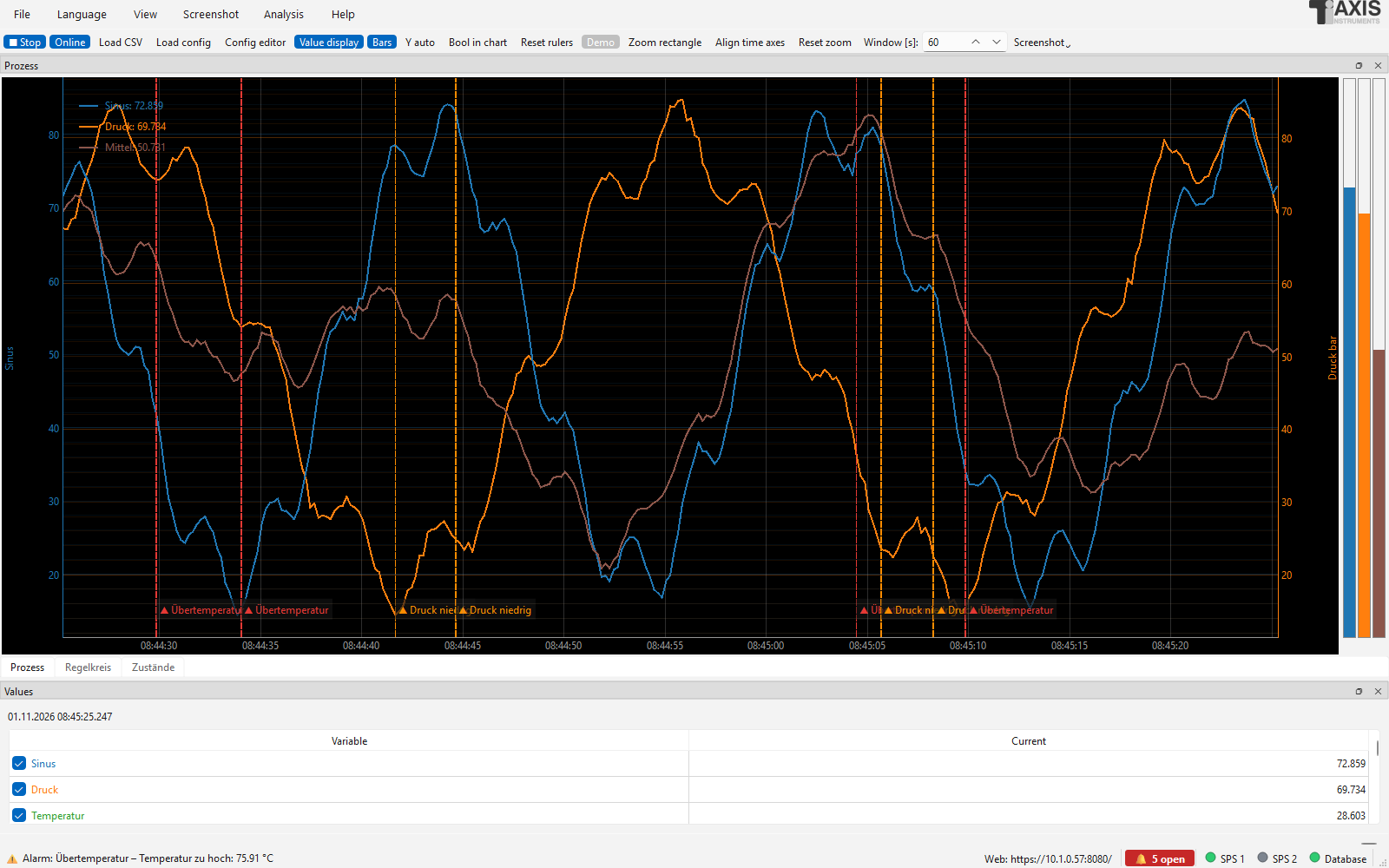
The main window of the logger with toolbar, charts, value table and status bar.
Toolbar (top):
Element |
Function |
|---|---|
▶ Start / ■ Stop |
Starts or ends recording and CSV logging. |
Online / Offline |
Switches between continuous display and review. |
Load CSV |
Opens saved CSV files for viewing (offline mode). |
Config editor |
Starts the configuration program. |
Value display |
Shows or hides the value table (right). |
Bars |
Shows or hides the narrow bars next to the charts. |
Y auto |
Active: all Y axes are scaled automatically and override fixed ranges. Inactive: the settings of the configuration apply. |
Bool in chart |
Additionally draws BOOL variables as a filled step line in the chart (depending on the Y axis). Default: off, BOOLs appear only as strips in the legend. |
Reset rulers |
Sets the two rulers (offline) to one third and two thirds of the visible time range. |
Demo |
Simulated values instead of a PLC (see Demo mode). |
Zoom rectangle |
Active: drag a region with the left mouse button; time and values of this chart are enlarged to it (see Zooming and time axes). |
Align time axes |
All charts show the time range of the chart used last again. |
Reset zoom |
Scale the Y axes as configured again and align the time axes. |
Screenshot |
Opens a list of the charts; the chosen chart is saved as PNG or SVG (see Screenshots of charts). |
Window [s] |
Width of the visible time window in seconds (1 to 604800). |
At the bottom of the window is the time scroll bar (active only in offline mode). The status line shows connection messages and the path of the saved CSV file.
The View menu contains the layout of the charts, a list for showing and hiding single charts and the switches for value display, values at the mouse pointer, trigger marks and bars. The Analysis menu contains XY chart, frequency analysis, PDF report and PID tuning.
Starting and stopping the recording
Press ▶ Start. The logger reloads the configuration, builds the charts and connects to the controllers.
Each controller is read at its own interval. The measurements are merged into rows and written to the CSV file.
■ Stop ends the recording and closes the file. When the program is closed, it stops automatically and – if the option is set – archives the current CSV file (see Limiting the file size and archiving).
If the connection is lost, the logger tries to restore it by itself and reports this in the status line. During the interruption there are gaps in the data – only for the variables of the affected controller; the others continue.
Reading, calculating the formulas and writing the CSV file run in separate threads, independent of the user interface. The display fetches a section of the data only about ten times per second and does not redraw invisible curves; this keeps operation smooth even with many variables.
File menu of the logger: Load config … (Ctrl+O, file dialog for a
configuration file with any name), Reload configuration (F5), Config
editor, Connect to logger (client) … (Ctrl+K, Logger as client), Load CSV, Join CSV files and save …, Load from database …,
Export values (CSV/Excel) …, Web server address …, Event log …, Note to
the event log … and Exit. The window title shows the project name and the
configuration file.
Status LEDs of the connections

Status LEDs in the status bar: green, yellow, red, grey.
In the status bar an LED with the controller’s name shows the connection state of each controller:
Colour |
Meaning |
|---|---|
grey |
Controller not active (disabled or recording stopped). |
yellow |
Connection is being established. |
green |
Connected, reading. |
red |
Connection or read error; the logger tries again. |
The LED’s tooltip shows the status message (for errors the error text) and the cycle time of the last read request. The web server shows the same LEDs.
Online mode
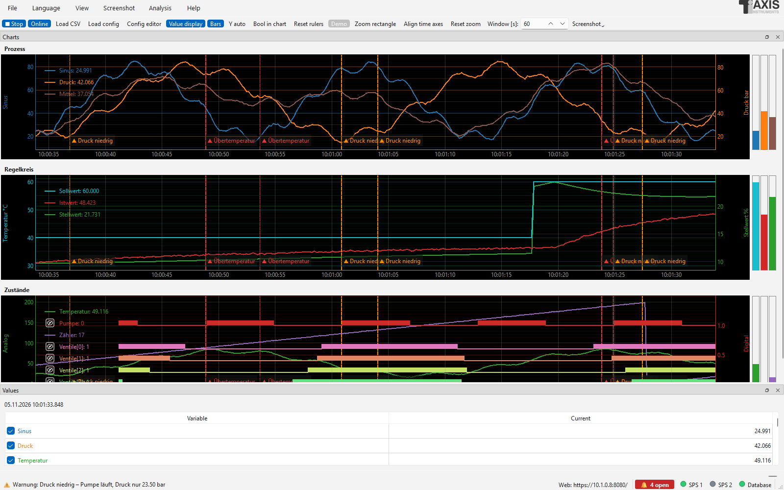
Online mode: continuous display of the last seconds.
In online mode the time axis follows the newest data. The last N seconds are always shown (setting Window [s]). The value table shows the latest measurement in the column Current. The recording continues independently of the display.
Values at the mouse pointer: When the mouse is over a chart, a dashed vertical line appears at the nearest measurement. A box next to it shows its time and the values of all visible variables of this chart (including BOOL variables); dots mark the values on the curves. If the mouse stays still, line and values move along with the new measurements. When the mouse leaves the chart, the display disappears. To switch off: View › Values at mouse pointer (online) (the setting is remembered). In offline mode the rulers take over this task.
Zooming with the mouse: In online mode, too, the time axis of a chart can be zoomed with the mouse wheel (or by dragging with the right mouse button); the new width applies to this chart only, the right end keeps following the newest values. More under Zooming and time axes.
Zooming and time axes (online and offline):
The mouse wheel, dragging with the mouse and the zoom rectangle only affect the chart under the mouse pointer. So each chart can show a different time range, e.g. one hour at the top and a few seconds below.
Zoom rectangle (toolbar, toggle): drag a region with the left mouse button – the time axis and all Y axes of the chart are enlarged to it. When it is off, the left mouse button moves the time axis.
Align time axes: all charts take over the range of the chart used last. A new entry in Window [s] aligns them as well.
Reset zoom: Y axes as configured again (or Y auto) and time axes aligned.
Window [s] and the scroll bar show the range of the chart used last. The scroll bar moves all charts together; each keeps its width.
Offline mode
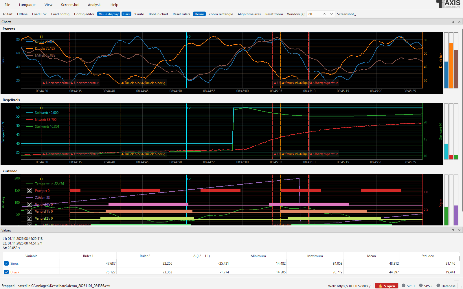
Offline mode: review with scroll bar.
In offline mode the display is frozen and you can go back in time:
Time scroll bar at the bottom: scroll through the recorded data.
Mouse: drag in the chart with the mouse button pressed to move the time axis, and zoom with the mouse wheel – each only in this chart (see Zooming and time axes). Scroll bar and Window [s] follow automatically.
Window [s]: width of the visible time range.
Note
When switching to offline mode, a snapshot of all data measured so far is taken. If the recording continues, newer data only appears when you switch from Online to Offline again.
The memory in the program is limited to about 300,000 data points; older points are then removed from the display. The CSV file always contains all data.
Rulers (offline)
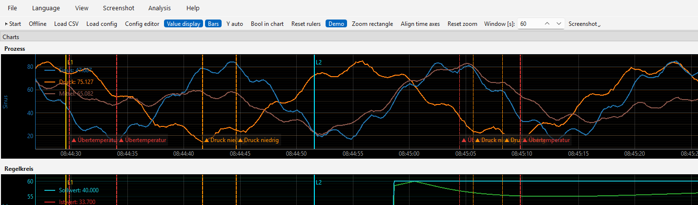
Two rulers with time and difference display.
In offline mode two vertical rulers appear in all charts: L1 (yellow) and L2 (cyan). Both can be moved with the mouse and are synchronized across all charts.
The value table then shows:
Column |
Content |
|---|---|
Ruler 1 |
Value of each variable at the time of L1. |
Ruler 2 |
Value of each variable at the time of L2. |
Δ (L2 − L1) |
Difference of the two values. |
Minimum, Maximum, Mean, Std. dev. |
Statistics of all measurements between the two rulers. |
Above the table the times of L1 and L2 and the time difference Δt in seconds are shown. The nearest measurement in time is used (no interpolation).
Trigger marks on the time axis
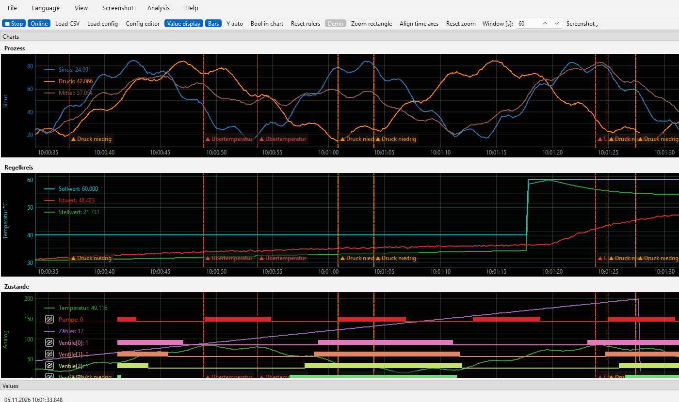
Trigger marks: alarm (red), warning (orange), recording by trigger (green), note (grey).
Events from the event log appear in all charts as a vertical dashed line with a short text at the bottom of the time axis (▲ name of the trigger): red = Alarm, orange = Warning, blue = Info, green = start of a recording by trigger, grey = note. The tooltip shows time, text and the times of going and acknowledgement. The marks are shown online and offline, also when displaying a loaded CSV file or a database time range (from the event log of the configuration). With very many events in the visible range at most 150 are shown. To switch off: View › Trigger marks on the time axis.
Pages, charts and layout
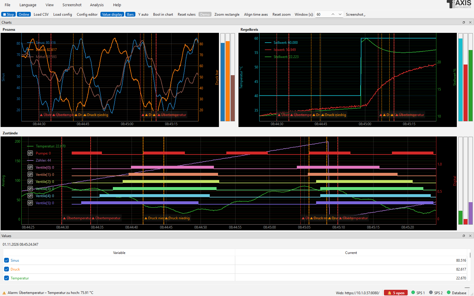
Charts of one page arranged as a grid.
The charts are placed on pages. A page is a dock window or a tab and can contain several charts:
Without page entries in the configuration, all charts are on one common page Charts. In Tabs mode each chart then gets its own tab.
With the field Page (tab) in the configuration you decide yourself which charts share a page (same page name = same page). This way you can create e.g. the tabs Process and Alarms with several charts each.
Minimum height and scroll bar: Each chart has a minimum height. If not all charts of a page fit into the window, a scroll bar appears on the page. In Side by side mode a minimum width with a horizontal scroll bar applies accordingly.
Layout of the pages (menu View › Layout):
Mode |
Effect |
|---|---|
Stacked |
Pages lie one above the other; the charts of a page are stacked. |
Side by side |
Pages lie side by side; the charts of a page are also side by side. |
Tabs |
Each page is a tab; the charts of a page are stacked. |
Layout of the charts on a page (menu View › Charts on the page): Automatic follows the layout of the pages; Stacked and Side by side force one column or one row; Grid arranges the charts in rows and columns. The number of columns is set with View › Grid columns (Automatic chooses about the square root of the number of charts, i.e. three columns for six charts). A last single chart fills the remaining row. The default is set in the configuration (tab Display).
The layout can be adjusted further by drag & drop:
Pages: grab the title bar of a page and drag it to the edge of another page (next to or above it) or onto its centre (as tab). Double-clicking the title bar detaches the page as a floating window.
Charts within a page: grab the title line of a chart (bold, above the chart) and drag it onto the title line of another chart on the same page. The chart is inserted at that position.
Pages can be hidden and shown again via View › Pages / charts. The page layout adjusted by drag & drop is kept when starting again within the same program session, as long as the page names and the mode stay the same. After restarting the program the default layout applies again.
All charts share the same time axis.
Legend with live values
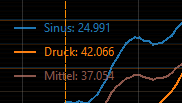
Legend with live values; one curve is highlighted, one hidden.
The legend in each chart shows the current value after the name of each variable,
in the variable’s colour, e.g. Temperature: 51.234. Online this is the latest
measurement, offline the value at ruler 1.
Highlighting a curve: a left click on the name (or sample) of a curve in the legend highlights it: the curve is drawn thicker and in the foreground, the name appears in bold, all other curves of the chart are dimmed. Clicking the same name again removes the highlighting; clicking another name moves it.
Hiding and showing a curve: right-clicking the name of a curve in the legend opens a menu with Hide curve or Show curve and Show all curves of this chart. Hidden curves appear grey in the legend with the addition (off). The tick in the value table stays in sync. The choice is kept when the layout changes.
Screenshots of charts
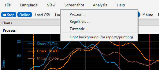
Menu “Screenshot” with choice of chart and light background.
Single charts can be saved as an image:
Click Screenshot in the toolbar (or in the Screenshot menu) and choose the chart.
In the save dialog choose file name and format: PNG (bitmap) or SVG (vector graphic). The format results from the file extension or the chosen file type.
The screenshot contains the chart exactly as displayed: curves, all Y axes, legend, bars and, in offline mode, the rulers. PNG files are created with double resolution. The SVG file is drawn from the measurement data itself (axes with ticks, grid, time axis, curves, BOOL traces, rulers with labels and legend with values) and can be scaled without loss and edited further, e.g. in Inkscape or office programs. If the chart is in a hidden tab, it is brought to the front automatically.
For reports and printouts, the option Light background (for reports/printing) can be switched on in the Screenshot menu. The screenshot is then saved with a white background and dark text; rulers are drawn in darker colours. The screen display itself stays unchanged. The setting applies to the current program session.
Value table (value display)
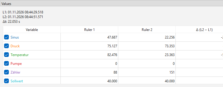
Value table with current values (online) or ruler values (offline).
The table on the right lists all variables for which value display is enabled in the configuration.
The name is shown in the variable’s colour. Hovering over the name shows the address (for calculated variables the formula).
With the tick in front of the name you hide or show the variable’s curve in the chart (alternatively by right-clicking in the legend).
The columns change with the mode (Current online, Ruler 1 / Ruler 2 / Δ offline).
Offline the table also shows the statistics between the rulers: Minimum, Maximum, Mean and Std. dev. (sample standard deviation, like
STDEVin Excel). All data points from the one at ruler 1 to the one at ruler 2 (inclusive) are taken into account; missing values are skipped. For BOOL variables the mean is the share of time the signal was on (0.25 = 25 %). The values follow every movement of the rulers.
Y axes and scaling
Each Y axis is labelled in the colour of its first variable.
Axes with auto scaling adapt to the data visible in the time window. Axes with fixed limits keep their range.
The Y auto switch in the toolbar temporarily overrides all fixed ranges. When it is switched off again, the settings of the configuration apply.
Bars for current values
Next to each chart a narrow bar per variable shows the current value (width adjustable: configuration › Display › Bar width). The scaling corresponds to the variable’s Y axis. In offline mode the bars show the values at ruler 1. Move the mouse over the bars to see names and values as tooltip.
BOOL variables
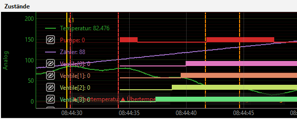
BOOL signals: line at 0, upward strip at 1, next to the legend rows.
Boolean variables are displayed independently of the Y axes:
In the legend name and value are listed one below the other like the analogue curves. Next to each BOOL entry, at the height of its legend row, a line on the base line (value 0) or an upward strip (value 1) in the variable’s colour runs across the width of the chart, like a digital signal. Like a curve it covers the displayed time range (online the last N seconds, offline the visible section). This way several BOOL variables can be compared at a glance without covering the chart.
As a curve BOOLs are not drawn by default (they would otherwise depend on a Y axis). With Bool in chart in the toolbar they additionally appear as a transparently filled step line.
In the value table the cell is filled in the variable’s colour for value 1 and empty for value 0.
Hidden BOOLs (right click in the legend) and highlighted BOOLs (left click) are dimmed or drawn with a thicker strip. The SVG export and the web server (where the name is shown in the row of the strip) show the BOOL signals in the same way.
Demo mode
Demo mode creates simulated values without a PLC being connected:
Activate Demo in the toolbar.
Press ▶ Start.
The variables of your configuration are supplied with test signals (REAL: sine with
noise, BOOL: square wave, integers: sawtooth). If nothing is configured yet, demo mode
creates example charts with several Y axes, a BOOL signal and a control loop for the PID
tuning. The switch is locked during recording and is not saved. The demo data is stored
as demo_YYYYMMDD_HHMMSS.csv.
Web server (charts in the browser)
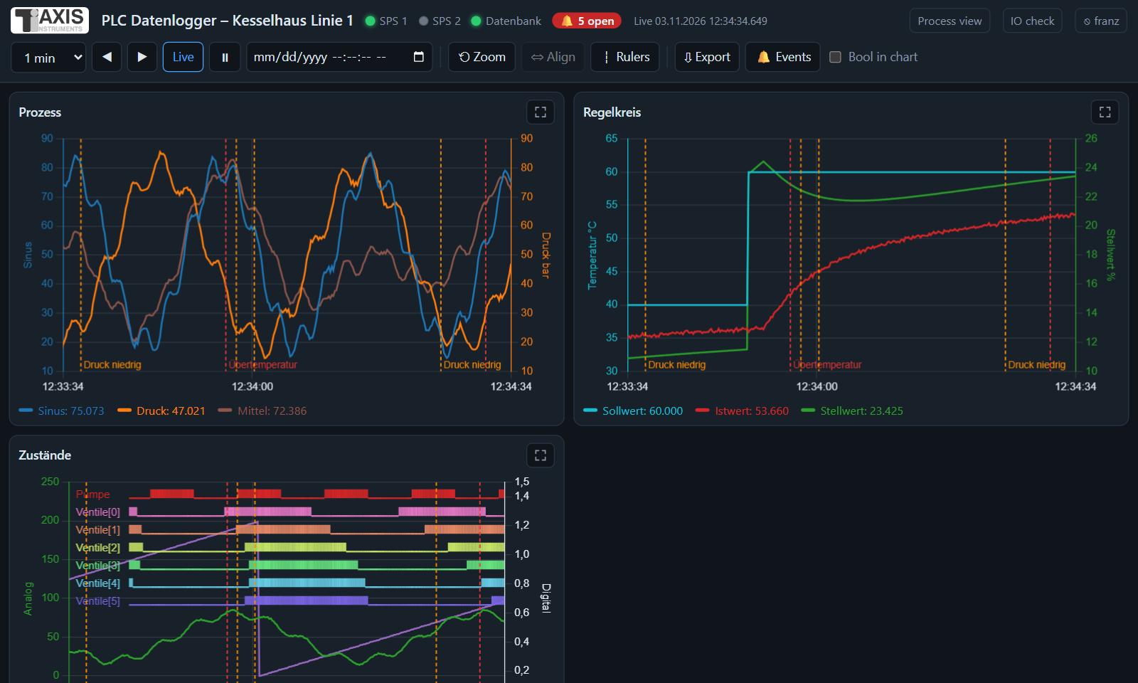
The charts in the browser of a tablet.
With the option Start web server (tab Web server & headless) the logger provides the charts as a web page. It can be opened with any browser in the network, e.g. on a tablet or smartphone – also in headless operation.
Address:
http://<IP address of the computer>:<port>/(default port 8080). The logger shows the address under File › Web server address … – together with a QR code: scan it with the smartphone camera instead of typing (with the access code if no login is set up). It is also written to the log at startup. The firewall may have to allow the port.Access code: If a code is entered in the tab, the page is opened with
http://…:8080/?token=CODE. Without code and without login anybody in the network can watch. There are no control functions; with write access events can be acknowledged, notes entered and the process view edited (see HTTPS and login).HTTPS and login: see below.
Process view: tiles with values, gauges and lamps under
/prozess, see Process view.Logos: customer logo and logo of the configuration (tab Display) appear in the header of the pages (charts, process view, login); empty fields = no logo.
Language: the pages (charts, login, process view, IO check) appear in the language set in the program (menu Language), e.g. English.
Display: The page shows the charts per page (tab) with Chart.js, with several Y axes, BOOL signals as step lines and status LEDs of the controllers. The display adapts to the screen size.
Operation: Live shows the latest time window; ◀ ▶ pages back in time (history), Pause stops the display. Tapping a legend entry highlights a curve, a long press or double-click hides it. Zoom, rulers, history from the database, export and events: see Analysing in the browser.
Full screen: The button at the top right of a chart (or a double-click into the chart) enlarges it to the whole window; the header with time window, ◀ ▶, Live and Pause stays visible and usable. Where the browser allows it, it also switches to real full screen (without address bar). Back to the normal display: the same button, double-click,
Escor the browser’s back button or gesture. In full screen more points are loaded (to match the width).Chart.js: The library is served from
web_static/chart.umd.js(the installer contains it). If the file is missing, the browser loads it from the internet instead (jsdelivr); in a closed network put the filechart.umd.js(Chart.js 4) into the folderweb_staticmanually.
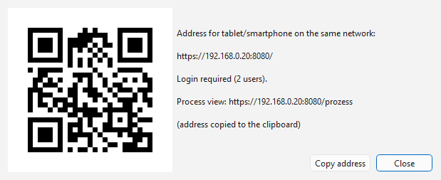
File › Web server address …: address with QR code for scanning.
The server transfers only the visible data, reduced to the screen width (minimum and maximum per section are kept), and compresses it.
Analysing in the browser
The web page offers the most important analyses of the logger – on PC, tablet or smartphone, without installation. One logger records (e.g. headless on a Raspberry Pi), any number of browsers show the same data.
Zoom: The mouse wheel over a chart (or two fingers on a tablet) stretches or compresses the time axis of this chart, two fingers also move it. Dragging a range with the mouse zooms to the chosen section – dragging vertically as well zooms the Y axes too. The chart then has an own time axis (note above the chart) and no longer follows Live. ⇔ Align applies the time range of the selected chart (blue frame) to all, ⟲ Zoom resets all charts (live, Y axes as configured).
Rulers: ┆ Rulers shows two vertical rulers and pauses the display. Dragging a ruler or clicking/tapping into the chart sets the nearer ruler. The legend shows the values at ruler 1 and 2 and the difference per variable, the line below the buttons both points in time and the distance.
History from the database: The logger keeps the latest values in memory (up to 300,000 rows). If a database is configured, the server fetches older periods from there – with ◀, the time window up to 7 days or the date/time field (jumps to this point in time). The header then shows Database. Long periods are read as averages; the browser needs no access to the database. Gaps (logger stopped) stay open in the chart.
Export: ⇩ Export saves the values of the displayed time range, between the rulers or of a free period as an Excel or CSV file (raw data, also from the database), optionally only the displayed curves. PDF report creates the report for the same period as in the logger (statistics, charts, events).
Events: 🔔 Events (or a click on the red open badge) lists events and notes of the last day up to year, optionally only open ones. ⌖ jumps to the point in the chart (ruler 1 at that time). With write access: ✓ Acknowledge (single or all) and ✎ Note … (at the time of ruler 1, otherwise now); the acknowledgement records the logged-in user. Events and notes appear as dashed marks in the charts.
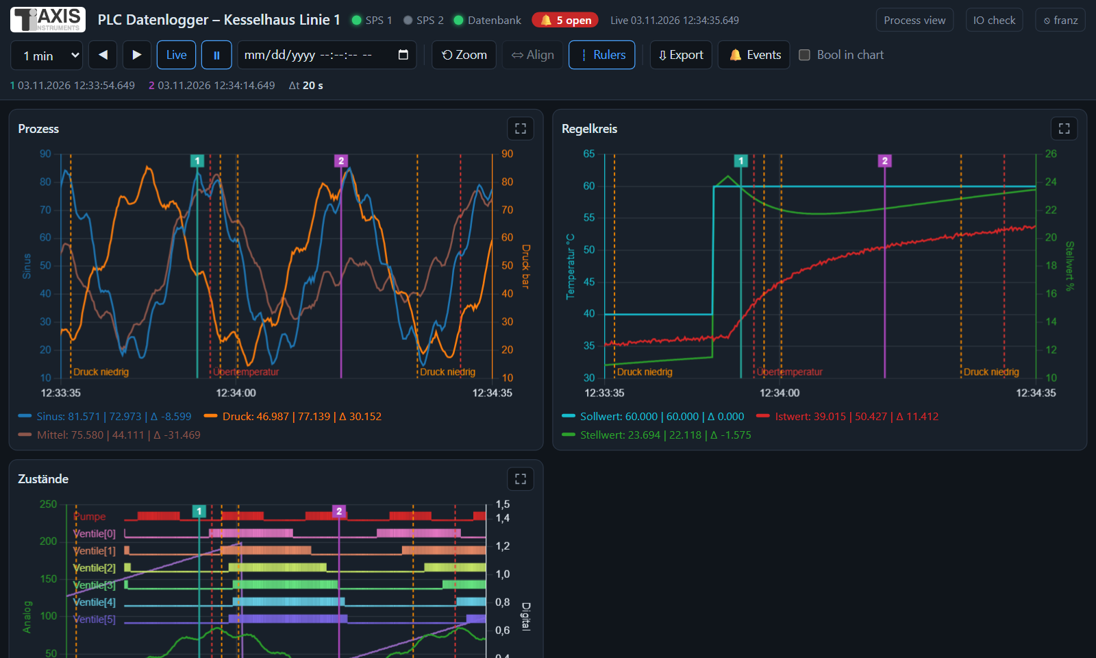
Rulers: values at both points in time and difference in the legend, event marks (dashed).
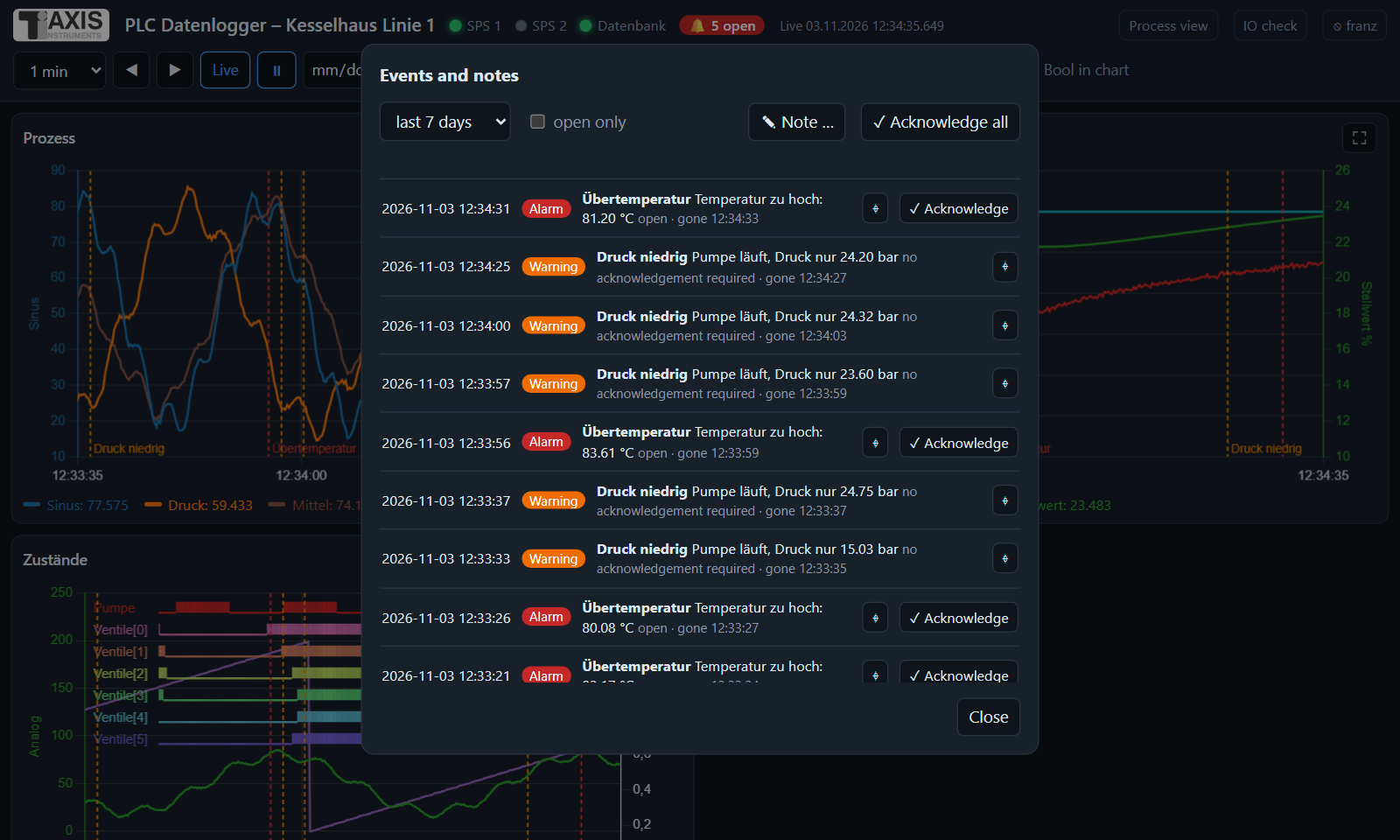
Events and notes: ⌖ jumps into the chart, acknowledging with write access.
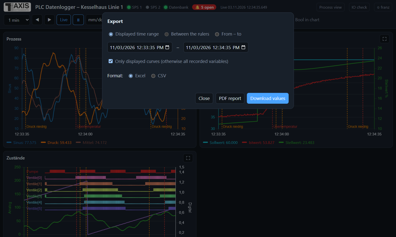
Export of the time range as Excel/CSV or PDF report.
HTTPS and login
Login page of the web server (smartphone).
HTTPS (tab Web server & headless, HTTPS (encrypted)): the page is then
reachable at https://<IP>:<port>/. Without a certificate of your own, the logger
creates a self-signed one at the first start (RSA 2048, valid for ten years, for
computer name, IP address and localhost; folder web_tls in the data folder). The
browser warns on the first visit because it does not know the issuer: compare the
fingerprint and confirm the exception. The SHA-256 fingerprint is shown under File ›
Web server address … (in headless operation it is in the log file). With a certificate
of the company CA (enter PEM files for certificate and key) there is no warning. Requires
the package cryptography (included in the installation).
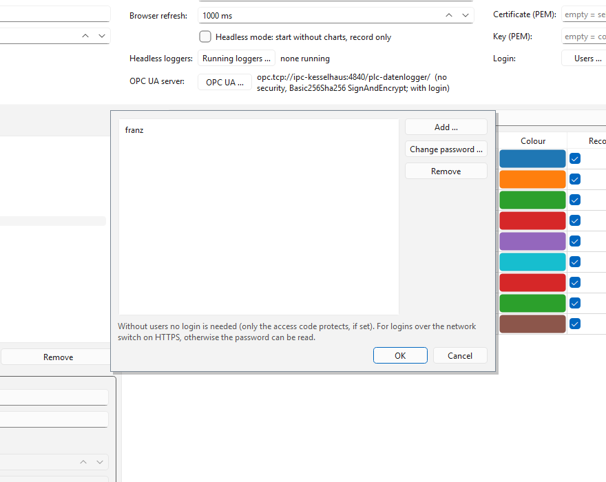
Creating web server users (configuration program, tab Web server & headless).
Login: Create users with Users … (name and password, at least 8 characters);
only a hash of the password (PBKDF2-SHA256) is stored, not the password itself. If at
least one user is configured, the browser first shows a login page; the login is valid
for 12 hours or until ⎋ Log out (top right of the page). After five failed attempts
the address is blocked for one minute. An additionally configured access code still
allows access without login (?token=CODE, e.g. for a permanently installed display).
Write access: The tick in front of the user name grants write access – acknowledge events, enter notes, edit the process view. Without the tick the user may only view and export. New users initially have no write access; users from older configurations keep it. Once users are set up, the access code alone only grants read access; without users, anybody with access may write. Next to Users …, ✎ marks the users with write access.
Note
Without HTTPS, passwords and measurements are transmitted unencrypted. Therefore use login together with HTTPS. For access from the internet, the server should also be behind a VPN or a reverse proxy.
Process view
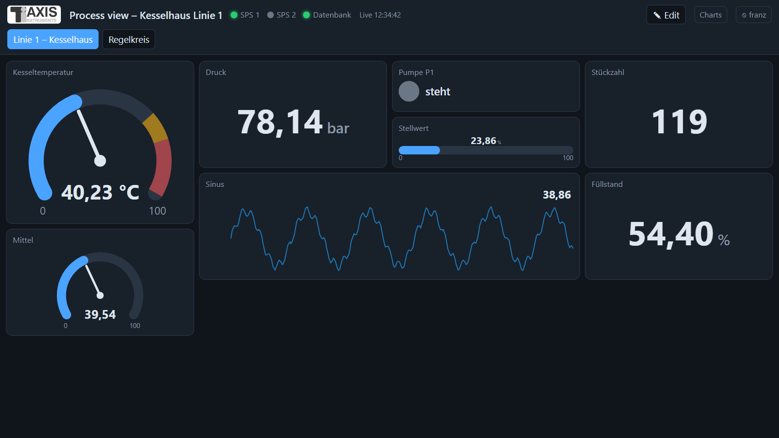
Process view: text, gauges, numeric values (pressure above the warning limit), status lamp, bars and short trend.
Besides the charts the web server offers a process view – an overview with large,
easily readable tiles, e.g. for a monitor in the control room or a tablet at the machine.
Open it with http://<IP>:<port>/prozess, the link Prozessbild at the top of the
chart page or in the logger with File › Process view in the browser (opens the
default browser of this computer). The web pages are in German.
Tile types:
Zahlenwert (numeric value) – large value with unit.
Zeigerinstrument (gauge) – arc from minimum to maximum, warning and alarm ranges in colour.
Balken (bar) – horizontal or (for a tall, narrow tile) vertical, e.g. a level.
Zustand (Lampe) (status lamp) – for BOOL signals: lamp with texts and colours for ON and OFF (optionally inverted).
Kurzverlauf (short trend) – line of the last seconds to hours (Zeitraum) with the current value.
Text / Überschrift (text / heading) – e.g. a plant section or a note.
For value, gauge, bar and trend, upper and lower warning and alarm limits can be entered: if one is exceeded, the tile turns yellow or red. Without a measurement (connection lost) — is shown. Several pages appear as tabs at the top. On a smartphone the tiles are stacked (two per row or a full row).
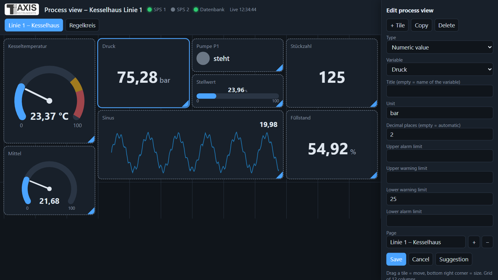
Editing: tile selected (blue), its properties on the right.
Editing: button ✎ Bearbeiten (on a PC or tablet). Dragging a tile with the mouse
moves it on the grid (12 columns), the bottom right corner changes its size; the arrow
keys move the selected tile, with Shift they change its size, Del deletes it. The
properties of the selected tile are on the right (type, variable, title, unit, decimals,
minimum/maximum, limits, colours, texts). + Kachel (add tile), Kopie (copy),
Löschen (delete), pages are added, deleted and renamed with +/−; Vorschlag
(suggestion) fills the page with one tile per variable. Speichern (save) stores the
layout, Abbrechen (cancel) discards the changes.
The layout is stored in the file
<configuration>.prozessbild.jsonnext to the configuration file (e.g.plant.prozessbild.json); the configuration program does not change it. Tiles refer to the name of a variable – if a variable is renamed, the tile shows “Variable fehlt” (variable missing) and has to be assigned again.Without a saved layout the page shows a suggestion (BOOL as lamp, otherwise value).
Who may edit: if users are set up (HTTPS and login), only logged-in users with write access – whoever opens the page with the access code only can view it but not change it (good for a permanently installed display). Without login anybody with access to the page may edit.
Logger as client
A logger can display the recording of another logger – for example a Raspberry Pi recording headless at the plant while a second logger in the office only displays and analyses. The client needs no configuration of its own and no connection to the PLC: charts, variables, page layout, window width and the names of the PLCs come from the recording logger, as do the values. On the server only the web server has to be enabled (Web server (charts in the browser)).
Connecting
in the start window Connect to logger …,
in the logger File › Connect to logger (client) … (Ctrl+K) or
from the command line
plc_logger.py --client https://logger-kessel:8080/ --benutzer chef(without an address only the dialog appears).
The dialog asks for the address (http:// or https://, host name or IP address
and port of the web server), user and password – or, without users set up, the
access code. Address and user are remembered for next time, the password never. If
the server uses a self-signed certificate, the client shows its SHA-256 fingerprint;
compare it with File › Web server address … on the server (headless: log file). Once
confirmed, the client remembers the certificate; if it changes later, the client refuses
to connect.
In the client
The display runs live (the client fetches the new rows at the refresh rate of the web server); on connecting, the last 30,000 rows come from the server’s memory. Offline view, rulers, zoom, value table, analysis (XY, FFT, PID), report, screenshots and Export values work as when recording yourself.
Load from database … and Show in chart (events) fetch older periods from the server – from its memory, before that from its database (long periods as averages). Back to the live display with Online.
The status LEDs show the state of the PLCs on the server; if the server cannot be reached they turn red and the client keeps trying.
Events: counter, event log and marks come from the server. Acknowledging and notes go to the server – only for users with write access (HTTPS and login).
If the server starts a new recording (e.g. with a changed configuration), the client reconnects on its own and rebuilds the display.
▶ Connect / ■ Disconnect replace start/stop. Not available are demo, configuration editor, IO check, web server and process view of the client – they belong to the recording logger. File › Disconnect (own configuration) or Load config … return to your own configuration.
The client writes no CSV files and nothing to the database; so there is only one recording and one data basis.
OPC UA server
The logger can provide its values itself as an OPC UA server – for a control system, MES, SCADA, Node-RED or another logger. This way, e.g. values from an S5 or a Modbus controller that cannot do OPC UA itself, and the calculated variables, can be used in an OPC UA network. The server is read-only.
Enable: configuration program, tab Web server & headless, OPC UA …:
Start OPC UA server – the server runs as long as recording runs (also in headless operation); at start the endpoint is shown in the status bar or the log.
Address (host) and port (default 4840). Endpoint:
opc.tcp://<computer>:4840/plc-datenlogger/. The firewall must allow the port.Update – how often changed values are taken over into the server (default 500 ms; faster than the sampling time of the controllers is pointless).
Security – one or more levels: None, Basic256Sha256 (sign or sign and encrypt), Aes128Sha256RsaOaep, Aes256Sha256RsaPss. For the encrypted endpoints the logger creates a self-signed certificate at the first start (folder
opcuain the data folder,server_cert.der); the client may have to accept it as trusted. Own certificate: enter the files.Access – Anonymous and/or Login with the web server users (the same names and passwords as in HTTPS and login). For a login an encrypted endpoint should be enabled, otherwise the password travels across the network in plain text.
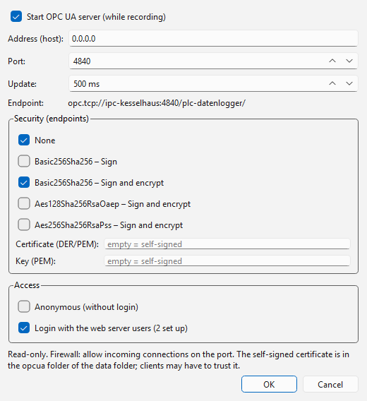
OPC UA server dialog: endpoint, security levels and access.
Address space (namespace urn:plc-datenlogger):
Objects
└─ PLC Datenlogger
   ├─ PLC 1                 one folder per controller with its variables
   │  ├─ Temperature        ns=2;s=Temperature   (Double; BOOL variables: Boolean)
   │  └─ …
   ├─ Calculated            calculated variables (formulas)
   ├─ Events                per trigger: Boolean, True while the event is active
   └─ Status
      ├─ PLC 1              Boolean: connection OK
      ├─ PLC 1_Text         status text of the connection
      ├─ Timestamp          time of the last measurement row
      └─ Recording          True while recording runs
The NodeId of a variable is its name (ns=<index>;s=<name>; the client gets the index
via the namespace urn:plc-datenlogger, usually 2). The folders Calculated, Events,
Timestamp and Recording are named in the language of the interface; their NodeIds do
not change. The source timestamp is the time of the measurement. If a variable has no
value (controller not reachable), it has the status BadNoCommunication. Clients can
read or subscribe to the values; only changes are reported.
Headless operation (recording only)
Without user interface the logger only records: reading from the controllers, formulas, CSV file, archiving, trigger recording, reports and – if enabled – web server. This saves resources and is suitable for continuous operation, e.g. as autostart program on an industrial PC.
Switching on: option Headless mode in the tab Web server & headless of the configuration, or command-line parameter
--headless. With--guithe user interface can be opened despite the headless mode being set. On Linux without a graphical session (systemd service, SSH) the logger always starts headless, even if the option is off.Messages (connection, errors, archiving) are written to the log file
plc_logger.login the program or data folder (rotating, several files).Exiting:
Ctrl+Cin the console window or the signal SIGTERM (stop service, Windows: close the window) exits cleanly: the CSV file is closed and – if the option is set – archived.Stopping from the configuration program: File › Show/stop headless loggers … or Running loggers … in the tab Web server & headless lists the running headless loggers (project, configuration, start time, computer, process ID, web server). Stop logger ends the selected one as cleanly as SIGTERM, within about one second – also on Windows and when the logger was started without a console. For this, every headless logger registers in the folder
laufendof the data folder; so the loggers shown are those running with the same data folder (same user or same portable folder). A logger running as a service under another user does not appear here; if a service restarts the logger automatically, stop the service itself (e.g.sudo systemctl stop <service>).The installed version contains the shortcut PLC Datenlogger (Headless, nur Aufzeichnung) in the start menu.
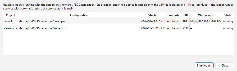
Running headless loggers in the configuration program.
Database recording
The measurements can be written to a database in addition to or instead of the CSV file – e.g. for evaluation with SQL or display in Grafana. The settings are in the configuration program in the tab Database; the CSV file is switched on or off with the tick Write CSV file in the tab Recording.
Field |
Meaning |
|---|---|
Database |
None, SQLite (file), MariaDB / MySQL, TimescaleDB / PostgreSQL, QuestDB, InfluxDB 3 Core, VictoriaMetrics or Prometheus (remote write). |
Server / port |
Host name or IP address of the database server; port default = 3306
(MariaDB), 5432 (PostgreSQL/TimescaleDB), 9000 (QuestDB), 8181 (InfluxDB 3) or
8428 (VictoriaMetrics) or 9090 (Prometheus). For QuestDB, InfluxDB, VictoriaMetrics
and Prometheus a complete URL may also be entered here, e.g. |
Database name |
Name of the database on the server. MariaDB/PostgreSQL: it must already exist, the program creates the table itself. InfluxDB 3: created if needed. Not relevant for QuestDB, VictoriaMetrics and Prometheus (one database per server). |
User / password |
Access data. The user needs the rights CREATE (at the first start) and INSERT.
The password is stored in plain text in the configuration file. QuestDB, InfluxDB,
VictoriaMetrics and Prometheus: user and password are sent with HTTP basic
authentication; without user the password is used as token (InfluxDB 3: token
|
SQLite file |
File name of the SQLite database; a relative path refers to the data folder of the program. |
Table |
Name of the table (default |
Write changes only |
A value is only written if it has changed, but at least every minute. Saves a lot of space for slowly changing values. |
Also write events and notes |
Additionally write trigger events and notes to the database (default: on, see Events in the database below). |
Delete after, Use at most |
Delete old values automatically (see Cleaning up old recordings): after n days (SQLite, MariaDB, PostgreSQL/TimescaleDB, QuestDB) or when the values take up more than n MB (SQLite only). |
Test database |
Connects, creates the table and reports the result. |
Storage … |
Shows the space used by the table and the whole database and the number of values. SQLite: file size, table, exact count. MariaDB and PostgreSQL/TimescaleDB: table and database, count estimated. QuestDB (from 8.2) and InfluxDB 3: table and count (InfluxDB without the values of the last minutes). Prometheus: only the whole database. VictoriaMetrics: whole database (space, values, bytes per value, retention, free space), the metric per project (values, variables, oldest value), the growth of the last 24 hours and the space needed at full retention estimated from it. |
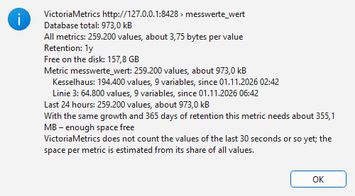
Storage … with VictoriaMetrics: whole database, per project and space needed.
Table structure (one row per value, “narrow” format):
Column |
Type |
Content |
|---|---|---|
|
SQLite: text, MariaDB: |
Time of the measurement in UTC with milliseconds |
|
Text (QuestDB: |
Project name from the configuration (several loggers can share a table) |
|
Text (QuestDB: |
Name of the variable |
|
Floating point number |
Measured value (BOOL as 0/1) |
Invalid values (e.g. during a connection failure) are not written. An index on
variable, zeit speeds up queries of single variables. With TimescaleDB the table
automatically becomes a hypertable (partitioned by time); if the extension is not
installed, a normal PostgreSQL table is created and the status line reports this.
QuestDB is addressed via its HTTP interface (default port 9000, the same port as the
web console): the values are sent in InfluxDB Line Protocol to /write, read-mode
queries to /exp. The table is created partitioned by day; from QuestDB 7.3 with
deduplication on zeit, projekt, variable – a batch sent again after a failure thus
does not create duplicate rows (older versions: without deduplication, the status line
reports this). An empty project name is stored as NULL.
InfluxDB 3 (Core or Enterprise) is also addressed via HTTP (default port 8181):
values in line protocol to /api/v3/write_lp, queries with SQL to
/api/v3/query_sql. The program creates database and table (tags projekt and
variable, field wert); in InfluxDB the time column is called time instead of
zeit. The same variable at the same time overwrites itself, so no duplicate rows
arise. If authentication is enabled (default in InfluxDB 3), enter the token
(influxdb3 create token --admin) in the field Password and leave User empty.
VictoriaMetrics stores time series instead of tables: each variable becomes a series
of the metric messwerte_wert with the labels projekt and variable. Writing
uses line protocol to /write, reading the Prometheus interface (read mode: raw data
via /api/v1/export, averages via /api/v1/query_range). VictoriaMetrics stores
timestamps with milliseconds and by default keeps data for one month only (command-line
parameter -retentionPeriod).
Prometheus stores time series like VictoriaMetrics (metric messwerte_wert, labels
projekt and variable). Writing uses remote write (/api/v1/write, protobuf
with snappy compression, no additional library); Prometheus must be started with
--web.enable-remote-write-receiver for this, otherwise the status line reports
“Remote write is not enabled”. Reading uses the HTTP interface (read mode: raw data hour
by hour via /api/v1/query, averages via /api/v1/query_range; first and last time
in the overview are accurate to about 1/2000 of the retention period). Prometheus only
accepts values per series in chronological order and at most about one hour old. It
rejects older values (e.g. written after a long outage); the logger discards such
batches, reports them (“… values rejected”) and counts them in the tooltip of the
database LED. Remedy: storage: tsdb: out_of_order_time_window: 1d in the Prometheus
configuration. The retention period is set with the command-line parameter
--storage.tsdb.retention.time (default 15 days).
Example queries:
-- Trend of a variable in the last hour (PostgreSQL/TimescaleDB)
SELECT zeit, wert FROM messwerte
 WHERE variable = 'Temperatur' AND zeit > now() - interval '1 hour' ORDER BY zeit;

-- Minute averages (TimescaleDB)
SELECT time_bucket('1 minute', zeit) AS minute, avg(wert)
  FROM messwerte WHERE variable = 'Temperatur' GROUP BY minute ORDER BY minute;

-- Latest values of all variables (MariaDB / SQLite)
SELECT variable, MAX(zeit) FROM messwerte GROUP BY variable;

-- Minute averages (QuestDB)
SELECT zeit, avg(wert) FROM messwerte WHERE variable = 'Temperatur' SAMPLE BY 1m;

-- Latest value per variable (QuestDB)
SELECT * FROM messwerte LATEST ON zeit PARTITION BY variable;

-- Minute averages (InfluxDB 3)
SELECT date_bin(INTERVAL '1 minute', time) AS minute, avg(wert) FROM messwerte
 WHERE variable = 'Temperatur' AND time > now() - INTERVAL '1 hour' GROUP BY 1 ORDER BY 1;
For VictoriaMetrics and Prometheus (PromQL, e.g. in Grafana):
messwerte_wert{variable="Temperatur"}                          # trend
avg_over_time(messwerte_wert{variable="Temperatur"}[1m])       # minute average
last_over_time(messwerte_wert{projekt="Anlage 1"}[1h])         # latest value per variable
Events in the database: With Also write events and notes the trigger events and the notes are stored in the database in addition to the event log (file) – e.g. for your own evaluations or as annotations in Grafana.
SQLite, MariaDB, PostgreSQL/TimescaleDB, QuestDB, InfluxDB 3: table table +
_ereignisse(i.e.messwerte_ereignisse), one record per event withzeit(came, UTC),projekt,id,trigger_name,prioritaet(priority),meldung(message),gegangen(went),quittiert(acknowledged),benutzer(acknowledged by or author of the note),notiz(note) andquittierpflicht(acknowledgement required) (InfluxDB: time columntime, went/acknowledged as text, plusdauer_s). When an event goes or is acknowledged, the record is updated. On start the logger synchronises all events of the log – including older ones and those acknowledged in the event viewer in the meantime.VictoriaMetrics, Prometheus: metrics table +
_ereignisse_aktiv(1 when coming, 0 when going; notes 1) and_ereignisse_quittiert(1, labelbenutzer) with the labelsprojekt,id,trigger_name,prioritaetandmeldung. Only new transitions are written; on start those of the last 10 minutes.A project name should be unique per logger: a record is identified by project, ID and time.
-- Open (not acknowledged) alarms
SELECT zeit, trigger_name, meldung FROM messwerte_ereignisse
 WHERE quittierpflicht = 1 AND quittiert IS NULL AND prioritaet = 'Alarm' ORDER BY zeit;

-- Most frequent events of the last 30 days (PostgreSQL)
SELECT trigger_name, count(*) FROM messwerte_ereignisse
 WHERE notiz = 0 AND zeit > now() - interval '30 days' GROUP BY 1 ORDER BY 2 DESC;
Operation:
Writing is done in a separate thread about once per second in batches; display and reading from the controller are not slowed down by this.
In the status bar (and in the web server) a separate LED “Database” shows the state; the tooltip gives the number of values written.
If the database cannot be reached, the values stay in memory (up to about 2 million values) and are written after reconnecting. Values not yet written when exiting are reported in the status line.
Drivers: SQLite is included in Python. MariaDB needs
PyMySQL, TimescaleDB/PostgreSQLpsycopg(pip install PyMySQL "psycopg[binary]"); both are included in the installer. QuestDB, InfluxDB 3, VictoriaMetrics and Prometheus need no library.For Grafana: create a data source MySQL or PostgreSQL (QuestDB: plugin QuestDB or PostgreSQL on port 8812; InfluxDB 3: InfluxDB with query language SQL; VictoriaMetrics and Prometheus: Prometheus); the time column is
zeit(InfluxDB:time, UTC).Grafana dashboard like in the logger: File › Export Grafana dashboard … in the configuration program saves a dashboard as a JSON file; upload it in Grafana via Dashboards › New › Import and choose the data source of the database. Taken over are the pages (as rows; layout Tabs: only the first one expanded), the arrangement of the charts (one below the other, side by side, grid), per chart the variables with colours, Y axes (left/right, fixed limits, axis name) and BOOL as a step line, the time range (Window [s]) and a selection Project at the top of the dashboard – so one dashboard serves several plants with the same configuration. Possible with VictoriaMetrics, Prometheus, TimescaleDB/PostgreSQL, MariaDB, QuestDB and InfluxDB 3 (not SQLite). After changes to charts, export again and overwrite on import. With Also write events and notes the dashboard contains the annotation Ereignisse (events): triggers and notes as a vertical line or region (comes to goes) in all charts, priority as tag (can be switched off at the top of the dashboard).
Up-to-dateness in Grafana: the dashboard queries again every 5 s (smallest default of Grafana). VictoriaMetrics does not show the last 30 s in queries yet. The logger’s web server is meant for the live display; if you still want Grafana faster, change it optionally: in Grafana
min_refresh_interval = 1s(grafana.iniorGF_DASHBOARDS_MIN_REFRESH_INTERVAL) and the refresh of the dashboard at the top right, for VictoriaMetrics the start parameter-search.latencyOffset=2s. Both lines are ready (commented out) indocker/docker-compose.yml.Test environment: in the folder
docker,docker compose up -dstarts TimescaleDB, QuestDB, InfluxDB 3 Core, VictoriaMetrics, Prometheus and Grafana with ready-made data sources (access data indocker/.env). SQLite files can be read with Grafana’s SQLite plugin.
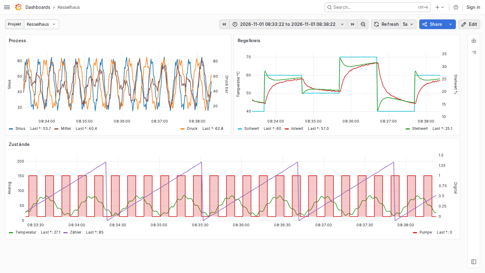
Exported Grafana dashboard (VictoriaMetrics): layout, axes and colours as in the logger, at the top the selection Project.
Read mode: displaying recordings from the database
In the logger, File › Load from database … (Ctrl+D) loads a freely chosen time
range from the database and displays it in offline mode – with rulers, value table,
screenshots and PID tuning as with a loaded CSV file. It reads from the database of the
loaded configuration; the database is only read, a running recording (also of another
logger) can continue writing meanwhile.
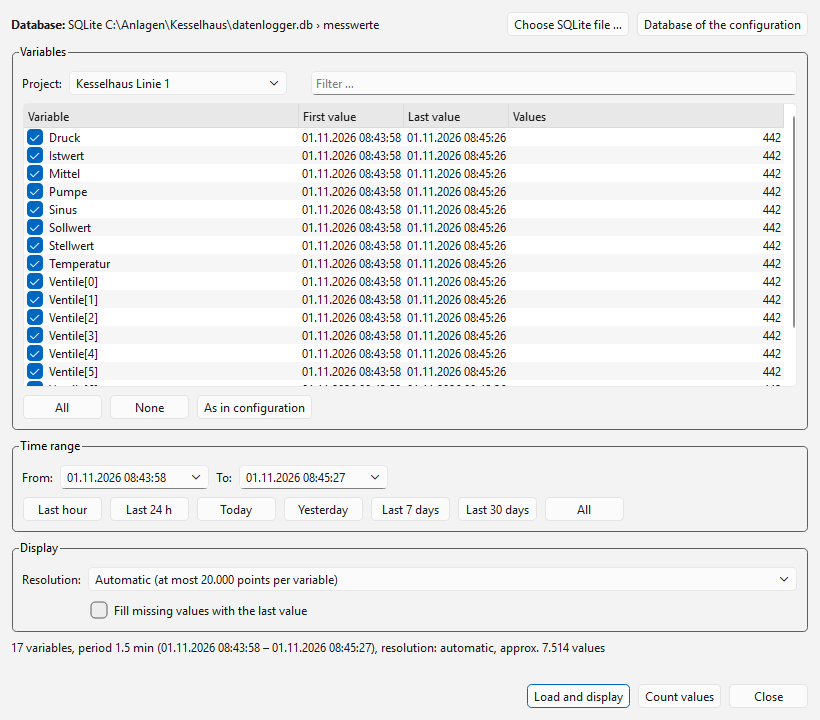
Dialog “Load from database”: choose variables, time range and resolution.
Area |
Meaning |
|---|---|
Database |
Shows the source. Choose SQLite file … reads any SQLite file instead (e.g. a copy from another computer); Database of the configuration returns. |
Project |
Project name under which the values were stored (default: project of the configuration). (all projects) combines variables of the same name of all projects. |
Variables |
All variables in the database with first and last time and number of values. Initially the variables of the current configuration are ticked. All, None, As in configuration and the filter field help with many variables. |
Time range |
From / To (local time) with calendar, or by button: Last hour, Last 24 h, Last 7 days, Last 30 days (each up to the last stored value of the chosen variables), Today, Yesterday, All. |
Resolution |
Automatic: raw data as long as there are at most 20,000 points per variable, otherwise averages on a suitable grid (1 s, 2 s, 5 s … 1 day). Raw data: every stored value. Average per 1 s … per day: fixed grids. The averages are computed by the database itself – so even months of data can be surveyed quickly. |
Fill missing values with the last value |
For recordings with Write changes only (preset there): a missing value means “unchanged”, the curve runs continuously. Without tick gaps appear. |
Count values |
Determines the exact number of values in the time range (above it there is an estimate from the variable list). |
Load and display reads the values in the background; the progress is shown at the bottom of the window, Cancel stops reading. Then the logger switches to offline mode. Colours, charts and axes come from the configuration; variables missing there appear in the first chart. The status line gives source, time range and resolution. A running recording is stopped when loading (as when loading a CSV file); ▶ Start begins a new one.
Notes:
Timestamps are stored in UTC in the database; they are displayed in local time.
With averages the timestamp is in the middle of the grid interval (e.g. 10:00:30 for 10:00:00 to 10:00:59). Minimum and maximum within an interval are not visible – choose raw data or a finer grid for short peaks.
To protect memory, the logger reads at most 20 million values at once; above that a note asks you to choose a shorter time range or averages.
With MariaDB and PostgreSQL the user only needs the SELECT right.
Triggers and event log
A trigger monitors a condition on the variables, e.g. {Temperatur} > 80. As
soon as it is met, the logger writes an entry with timestamp to the event log (a
text file). The number of events not yet acknowledged is shown in the logger’s status
bar; acknowledgement is done in the event viewer or in the browser (Analysing in the browser).
Creating triggers
Configuration program, tab Triggers & events → Edit triggers ….
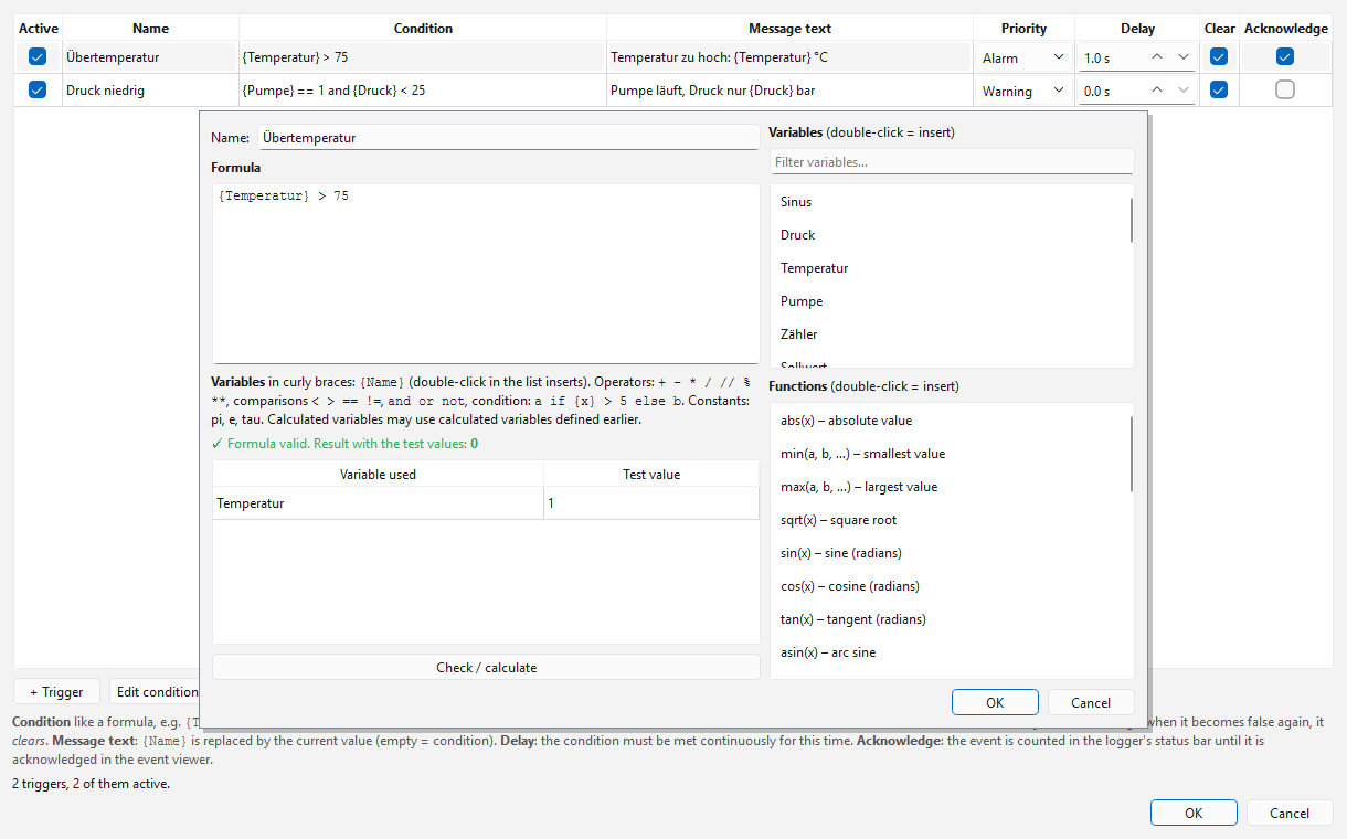
The trigger editor: one row per trigger, faulty rows are marked red.
Column |
Meaning |
|---|---|
Active |
Only active triggers are evaluated. Disabled triggers may also be faulty (e.g. after renaming a variable). |
Name |
Name of the trigger (unique, without |
Condition |
Expression as for calculated variables. Result not
equal to 0 = met. Examples: |
Message text |
Text of the entry. |
Priority |
Info, Warning or Alarm (colour in the viewer, filter). |
Delay |
The condition must be met continuously for this many seconds before the event is raised (suppresses short peaks). 0 = immediately. |
Clear |
Also log the end of the event (condition false again). |
Acknowledge |
The event must be acknowledged and is counted in the status bar until then. Without tick it is only logged. |
A trigger fires once per edge: only when the condition becomes false and then true again is a new event created. The triggers are checked with every measurement cycle – also in headless operation – and apply from the next start of the recording. In demo mode without own triggers there are two example triggers (Übertemperatur, Druck niedrig).
Event file
Field Event file in the same tab; empty = <CSV folder>/<CSV name>_ereignisse.csv.
The file is only appended to (never changed or archived) and can be opened with Excel
(semicolon, UTF-8):
ID;Zeit;Art;Trigger;Priorität;Text;Benutzer
17;2026-10-15 16:20:01.250;KOMMT;Übertemperatur;Alarm;Temperatur zu hoch: 81.37 °C;
17;2026-10-15 16:22:40.100;GEHT;Übertemperatur;Alarm;;
17;2026-10-15 16:25:12.000;QUITTIERT;Übertemperatur;Alarm;;mmuster
Art (kind) is KOMMT (raised), GEHT (cleared) or QUITTIERT (acknowledged);
rows with the same ID belong to the same event. For QUITTIERT the column
Benutzer (user) contains the Windows user name. - in the column Benutzer of a
KOMMT row means “no acknowledgement required”. The file format is the same in all
languages.
Display in the status bar

Red background: three events are not yet acknowledged.
On the right of the status bar the button 🔔 shows the number of open (not
acknowledged) events; with open events it is red. A click on it – or File → Event log
… (Ctrl+E) – opens the viewer. Each new event also appears as a message in the status
bar (⚠ Alarm: …). The counter also works without a running recording, e.g. if a
headless logger on the same computer writes to the file. In the web server “🔔 n open”
is shown at the top (tooltip: the open events); acknowledgement is only possible in the
viewer.
Event viewer and acknowledgement
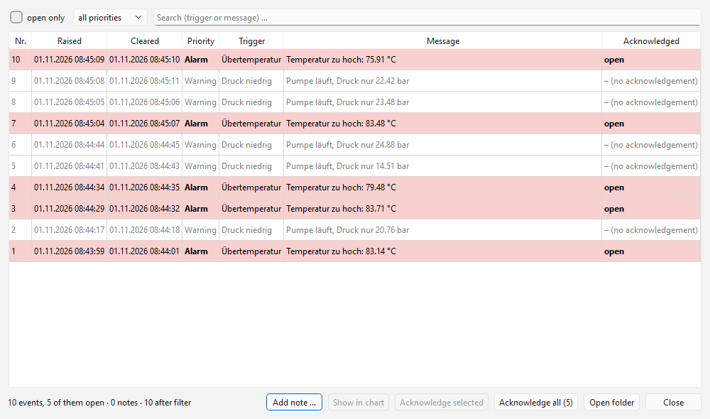
The event viewer: open events coloured by priority, completed ones grey.
The table shows the newest events at the top: number, raised, cleared, priority, trigger, message and acknowledgement (time and user or open).
Filters: open only, priority, search field (trigger or message).
Acknowledge selected (or double-click a row) acknowledges the selected events, Acknowledge all all open ones.
The display updates itself as soon as new events arrive (F5 = immediately).
Show in chart (button or right-click on a row, only in the logger): the logger switches to offline mode and shows the time range around the event, ruler 1 on the start (coming), ruler 2 on the end (going). If the values are no longer in memory, it loads them from the database of the configuration (if one is set; 10 minutes before and after the event), otherwise the matching CSV file from the CSV folder or the archive.
Open folder shows the event file in the file manager.
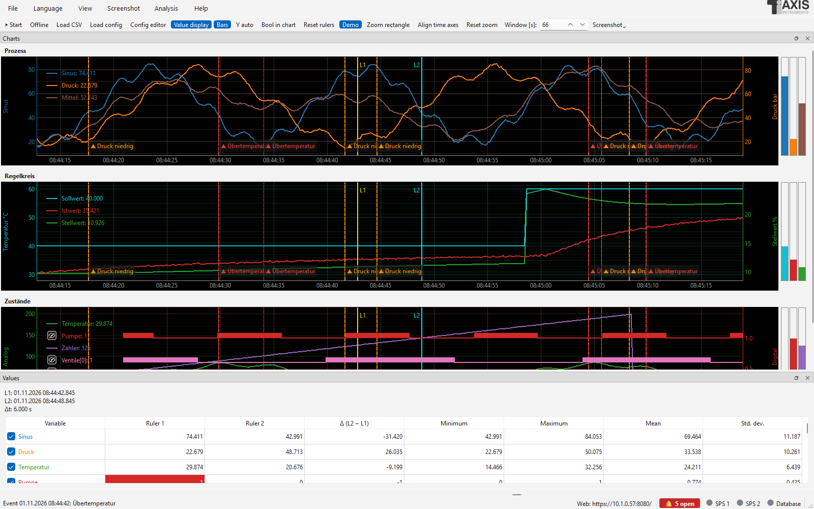
After “Show in chart”: time range around the event, ruler 1 on coming, ruler 2 on going.
The viewer can also be started on its own – e.g. next to a headless logger or on another computer with access to the file (network drive):
PLCLogger.exe --ereignisse                        (event log of the last used configuration)
PLCLogger.exe --ereignisse plant.json             (event log of this configuration)
PLCLogger.exe --ereignisse D:\logs\log_ereignisse.csv
The installed version has the shortcut PLC Ereignisprotokoll in the start menu for this. In the configuration program Show event log … opens the same viewer.
Notifications
When an event comes, the logger can pass it on immediately – by e-mail, into a Microsoft Teams or Slack channel, to any webhook (JSON), as a push message to the phone with the app ntfy or via Telegram. Set it up in the configuration program, tab Triggers & events, Notifications …; next to it you see whether and where notifications go.
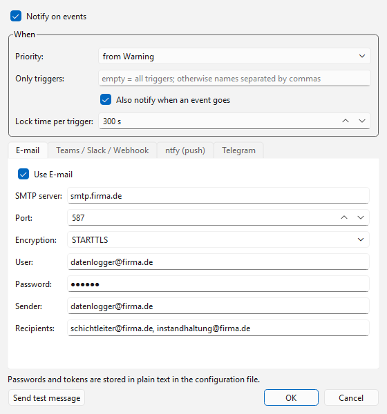
Notifications: at the top when to notify, below one tab per channel.
When to notify:
Notify on events – main switch.
Priority – from Info, Warning (default) or only Alarm.
Only triggers – empty = all; otherwise the names separated by commas.
Also notify when an event goes – an additional message when the condition is no longer met (only if the coming was notified).
Lock time per trigger (default 300 s) – if the same trigger comes again within this time, no further message is sent; the next message states how many were suppressed. Prevents message floods from a fluttering signal.
The message contains priority, trigger, message text, time, project and computer name.
Channels (one tab each, can be enabled individually):
E-mail: SMTP server, port (587 with STARTTLS, 465 with SSL/TLS, 25 unencrypted), user and password (empty = without login), sender and recipients (several separated by commas).
Teams / Slack / Webhook: Microsoft Teams (Workflows) – in the Teams channel under Workflows create the template “Post to a channel when a webhook request is received” and enter its address; the message appears as a card, alarms in red. Slack – address of an incoming webhook. Generic (JSON) – sends title, text, trigger, priority, type (KOMMT/GEHT), time, project and computer as JSON by POST, e.g. to Node-RED, Home Assistant or your own system.
ntfy (push): install the app ntfy on the phone and subscribe to a topic; enter the address with topic here, e.g.
https://ntfy.sh/plant-4711-xyz. Alarms arrive with the highest urgency. Onntfy.shanybody who knows the name of the topic can read along – choose a name that is hard to guess or run your own ntfy server (then enter an access token if needed).Telegram: create a bot with @BotFather (gives the bot token), send the bot a message and enter the chat ID (e.g. via @userinfobot).
Send test message sends a test via all enabled channels and shows ✓ or the error for each channel. Sending happens in the background, recording does not wait for it; errors (server not reachable, wrong login) are shown in the status bar or the log file. Notifications also work in headless operation – the computer needs access to the mail server or the internet for this.
Note
Passwords and tokens are stored in plain text in the configuration file. Make the file accessible to authorised persons only and use a separate account for e-mail.
Notes (own entries)
Besides the triggers, notes can be written by hand to the event log, e.g. “Valve V12 replaced” or “Setpoint changed to 65 °C” – so the same file later tells why a trend changed.
In the logger: File → Note to the event log … (Ctrl+M). In offline mode the time of ruler 1 is preset – so a point in the trend can be commented afterwards.
In the event viewer: Add note ….
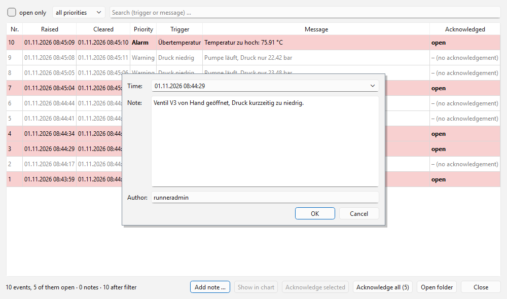
Time, text and author of a note.
Time (default: now), text (also multi-line) and author (default: Windows or Linux user
name) can be chosen freely. Notes are stored as kind NOTIZ in the file, appear in
the viewer with a green background and 📝 and need no acknowledgement. The filter
notes only shows only them.
18;2026-10-16 09:12:00.000;NOTIZ;Notiz;Notiz;Valve V12 replaced;mmuster
Recording by trigger (pre- and post-trigger)

Tab Recording: recording by trigger with start condition, pre- and post-trigger time.
Instead of recording continuously, the logger can write to the CSV file and database only when something happens – with the values before the event (pre-trigger) and after it (post-trigger). Typical applications: fault analysis, test cycles, batches.
Settings (configuration program, tab Recording):
Recording: By trigger with pre- and post-trigger time.
Start condition: a condition as for triggers, e.g.
{Druck} > 5,{Störung} == 1orabs(ddt({Kraft})) > 100; … opens the formula editor with variable list and check. All variables including the calculated ones can be used.Pre-trigger: this many seconds before the trigger are saved as well. For this the logger keeps the latest measurements in a ring buffer.
Post-trigger: saving continues this long after the condition has ended. If the condition becomes true again during this time, the capture is extended.
max.: maximum duration of a capture (unlimited = 0). After that the capture ends even if the condition is still met; the next one only starts after the condition has been false once.
Sequence: After the start the status bar shows ⏸ waiting for trigger. When the
condition becomes true, a capture begins (⏺ Capturing): a new CSV file
(<CSV name>_<date>_<time>.csv) with the pre-trigger values and all following values
up to the end of the post-trigger time. Each capture gets its own file; it stays in the
CSV folder. With a database, the same rows are written to the database. Start and end
are logged as event Aufnahme (capture; priority Info, no acknowledgement required)
in the event log and appear as a green trigger mark in the chart.
The display in the logger (and in the web server) always continues, also between the captures. If the start condition is faulty (e.g. unknown variable), the logger reports it and records continuously to be on the safe side.
Tip
Several captures can be joined into one file again with File › Join CSV files and save … (see Joining several CSV files).
PID controller tuning
If a chart shows a control loop – setpoint, process value and controller output – the logger calculates suitable controller parameters (Kp, Ti, Td) from the recorded data. To do this, it first identifies a model of the process and then applies proven tuning rules.
Switching on (configuration program)
Select the chart in the assignment tree and tick PID controller tuning under Properties of the selection. In the window Settings … you define:
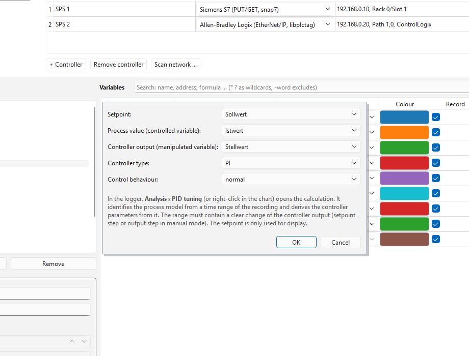
Assign setpoint, process value and controller output of the chart.
Field |
Meaning |
|---|---|
Setpoint |
Variable with the setpoint (optional, for display only). |
Process value |
Controlled variable (measured value), e.g. temperature. |
Controller output |
Controller output, e.g. valve position or heating power in %. |
Controller type |
PI (usually sufficient, insensitive to measurement noise) or PID. |
Control behaviour |
fast (aggressive, small margin), normal or robust (slow, safe even with a varying process). |
The assignment is suggested from common names (Soll/SP, Ist/PV, Stell/CV/Out …).
Recording data
The calculation needs a time range in which the controller output changes noticeably and the process value reacts to it:
Step of the controller output in manual mode (best): set the controller to manual, let the process settle, step the output by 5 … 20 % and wait until the process value is steady again.
Setpoint step in automatic mode: works as well, as long as the controller is not too sluggish and the output is not permanently at its limit (0 / 100 %).
The range should begin with a steady process and contain no large disturbances.
Calculating (logger)
Menu Analysis → PID tuning: <chart> … or right-click into the chart → Tune PID controller ….
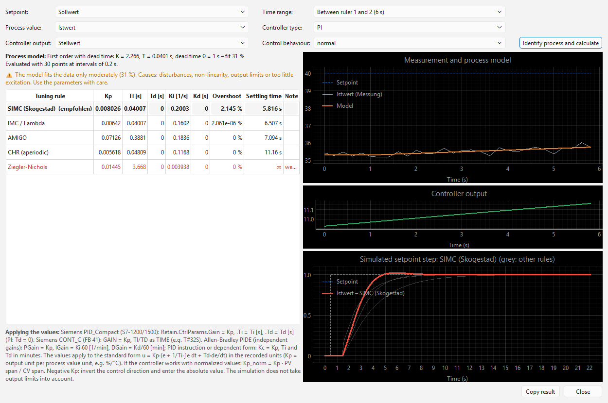
Left model and parameters, right measurement/model, controller output and simulated setpoint step.
Choose the time range: Between ruler 1 and 2 (offline mode, place the rulers around the step beforehand), Visible range or All data.
Click Identify process and calculate. The process model is shown at the top:
first order with dead time – gain K, time constant T, dead time θ (temperature, pressure, flow, speed …);
integrating process with dead time – integral gain Ki (e.g. level).
The fit states how well the model matches the measurement (100 % = perfect). Below about 50 % the parameters are uncertain; notes below name possible causes. In the chart on the right the model curve (orange) lies over the measured process value (grey).
The table shows the parameters according to several tuning rules; the first (bold) is the recommended one:
Rule
Properties
SIMC (Skogestad)
Recommendation: good setpoint tracking and disturbance rejection, little overshoot.
IMC / Lambda
Smooth, practically without overshoot; spares actuators.
AMIGO
Robust (Åström/Hägglund), good disturbance rejection.
CHR (aperiodic)
Chien-Hrones-Reswick, setpoint response without overshoot.
Ziegler-Nichols
Classic, fast, but poorly damped – for comparison only.
Columns: Kp (gain), Ti and Td in seconds (standard form
u = Kp·(e + 1/Ti·∫e dt + Td·de/dt)), plus the parallel form Ki = Kp/Ti and Kd = Kp·Td as well as overshoot and settling time (2 % band) from the simulation.At the bottom right the simulated setpoint step with the selected rule is shown (red; the others grey). Controller type and control behaviour can be switched in the window – the table is recalculated immediately.
Copy result puts the model and all parameters as text on the clipboard.
Notes
Kp applies in the recorded units (output unit per process value unit, e.g. %/°C). If the controller in the PLC works with normalized values, convert:
Kp_norm = Kp · process value span / output span.A negative Kp means: the process value falls when the output rises (e.g. cooling). Reverse the action in the controller and enter the absolute value.
The simulation does not take output limits into account. Introduce new parameters carefully and observe the control loop.
In demo mode the example configuration contains the chart Regelkreis with a simulated, deliberately sluggish controller (setpoint changes every minute) – after a few minutes of recording the tuning can be tried out.
Transfer to the controller: PIDE with independent gains:
PGain= Kp,IGain= Ki·60 [1/min],DGain= Kd/60 [min]. PIDE dependent form or PID instruction:Kc= Kp, Ti and Td in minutes (divide the values from the table by 60). PIDE computes in % of the rangesPVEUMax/MinandCVEUMax/Min– convert Kp accordingly.
Analysis: XY chart and frequency analysis
Both evaluations are available in the logger in the Analysis menu and work with the displayed data – during recording, offline or with a loaded CSV file or database time range. The time range can be chosen: Between ruler 1 and 2 (offline), Visible range or All data. The windows stay open next to the main window; Refresh fetches the data again. Save image … saves the chart as PNG, Save values (CSV) … the displayed values.
XY chart
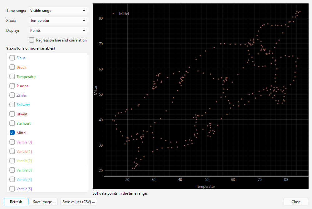
XY chart with regression line.
One or more variables (Y) against another variable (X) – e.g. pressure over stroke, force over distance or a characteristic curve. Choose the X axis, tick the Y axis variables in the list (colours as in the configuration). Display as Points, Line (in time order) or both. Regression line and correlation draws the regression line per Y variable and gives the correlation coefficient r and the line equation.
Frequency analysis (FFT)
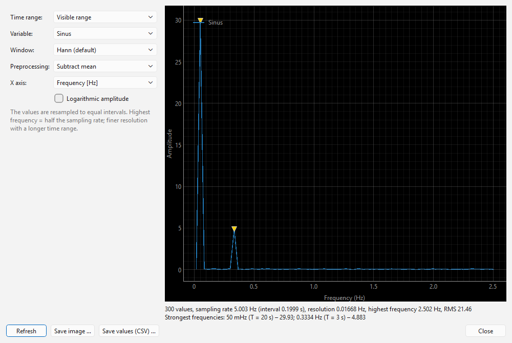
Amplitude spectrum with the strongest frequencies.
The amplitude spectrum of a variable, e.g. to find oscillations, hunting of a control loop or periodic disturbances. The measurements are first resampled to equal intervals (usual sampling interval); missing values are bridged.
Window: Hann (default), Hamming, Blackman, Flat-top (accurate amplitudes) or Rectangle (no window).
Preprocessing: subtract the mean or a linear trend (otherwise the DC component hides the low frequencies).
X axis: frequency in Hz or period in s (logarithmic); amplitude optionally logarithmic.
Below the chart the sampling rate, resolution (= 1 / duration of the time range), highest frequency that can be shown (half the sampling rate) and the strongest frequencies with period and amplitude (yellow triangles in the chart) are given. A sine of amplitude A appears with about the height A.
Tip
For a fine frequency resolution choose a long time range; for high frequencies a short interval of the controller (at 100 ms at most 5 Hz are visible).
PDF reports
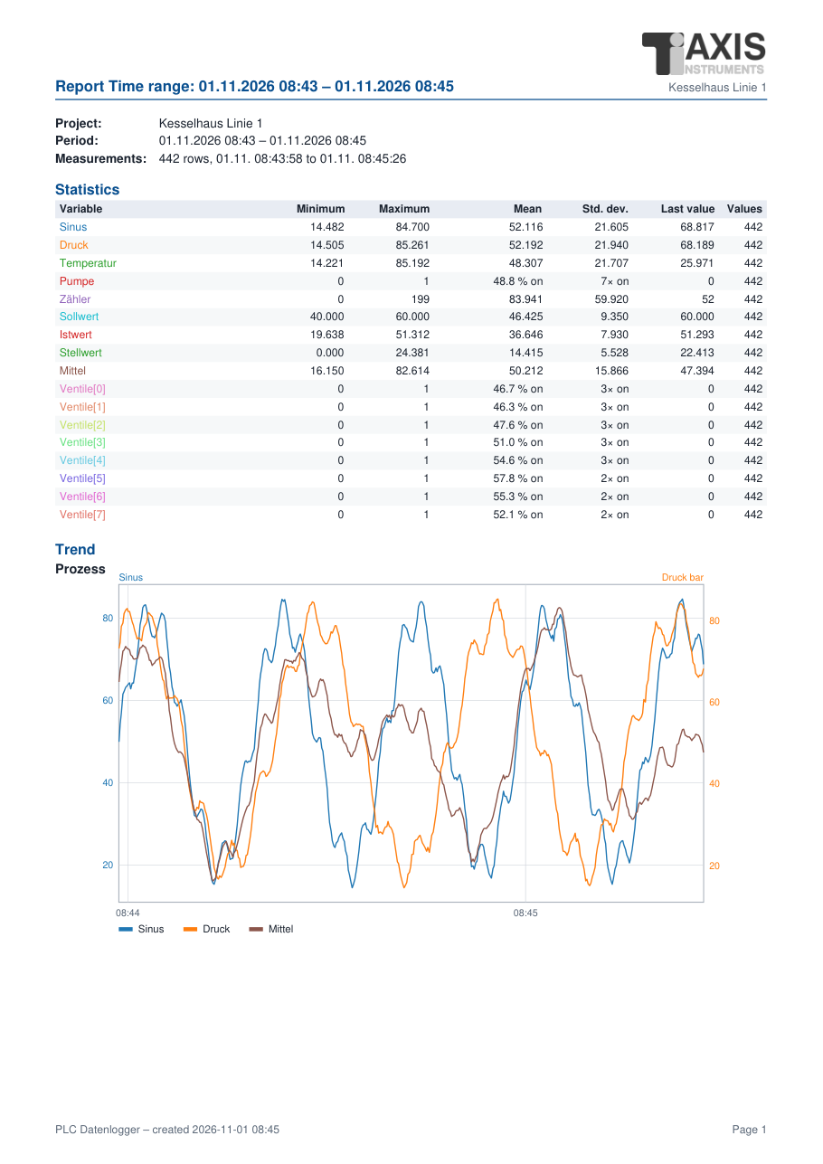
First page of a PDF report.
A report summarizes a period on a few pages:
Header: project, period, data basis (number of measurement rows, first and last measurement); above it the customer logo and logo from the configuration (tab Display), if entered.
Statistics per variable: minimum, maximum, mean, standard deviation, latest value and number of valid values; for BOOL variables the share of time with value 1 (on time) and the number of switch-on events.
Trend of every chart of the configuration with its Y axes; BOOL variables as traces below the chart (height = share of time with value 1). Peaks are preserved (minimum and maximum per time section).
Events and notes of the period from the event log.

Tab Reports (PDF) in the configuration program.
Automatic (configuration program, tab Reports (PDF)): at the end of every shift,
day, week or month the logger writes the report to the folder berichte
(name <CSV name>_bericht_<period>_<start>.pdf) – also in headless operation. For this
it collects the statistics and a condensed version of the trend during the recording,
regardless of how many measurements it keeps in memory. When stopping or exiting, a
partial report (suffix _teil, title “incomplete”) is created for the period
begun. Shifts start at the configured times; day, week (Monday) and month at the day
start.
Manually: Analysis › Create PDF report … – choose the time range (between the rulers, visible, all), confirm the file name; the report then opens in the PDF viewer.
The PDF files are created without additional programs (standard font Helvetica, vector graphics). The texts in the report follow the language of the program.
IO check (commissioning)
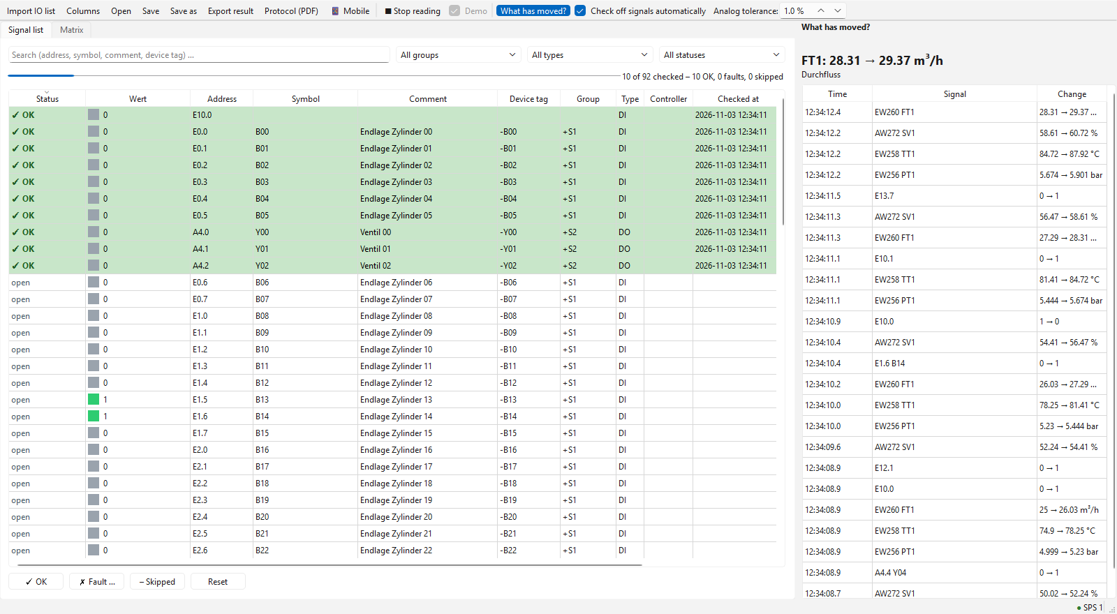
The IO check window: signal list with live values and status, on the right “What has moved?”.
The IO check helps to test all inputs and outputs of a plant during commissioning: every signal of the IO list is shown live and checked off; what has just moved is shown at the top, and swapped signals are noticed immediately. The IO check reads from the controllers of the configuration itself – no recording needs to be running.
Opening:
as a program of its own,
PLCIOCheck.exe(start menu PLC IO-Check, optionally also on the desktop). The start screen lists the recently used test files (*.iocheck.json) and configurations; a configuration starts a new test file with its controllers, Demo starts with simulated values;in the configuration program File › Start IO check with this configuration;
in the logger Analysis › IO check …;
Linux/AppImage or from the source code:
--iocheck(plc_logger.py --iocheck), optionally with a configuration or a test file.
▶ Start reading (F5) connects to the controllers; with Demo the signals are simulated (to try it out without a controller).
Note
The IO check only reads. Outputs are switched as before with the engineering tool (watch/force table) or the program and checked off in the IO check.
Importing the IO list
Import IO list … reads a CSV, Excel or ODS table (LibreOffice), e.g. from EPLAN, the TIA Portal tag table (export to Excel) or an own list. The columns are recognized by their heading (case does not matter):
Field |
Recognized headings (selection) |
|---|---|
Address (required) |
Address, Adresse, Logical Address / Logische Adresse, Operand, Tag name, NodeId |
Symbol |
Symbol, Name, Variable, Signal |
Comment |
Comment, Kommentar, Description, Function |
Device tag |
BMK, Device tag, Betriebsmittelkennzeichen |
Group |
Group, Cabinet, Station, Module, Gruppe, Schrank |
Type |
Type, Kind, Signal type (DI/DO/AI/AO, Input/Output …) |
Data type |
Data Type, Datentyp (Bool, Int, Word, Real …) |
Controller |
Controller, PLC, Steuerung – name of the controller in the configuration; empty = first |
Measuring range |
Range / Messbereich (e.g. |
If type and data type are missing, they are derived from the address: E0.0/%I0.0
= digital input, A4.0/%Q4.0 = digital output, EW256/%IW256/PEW256 =
analog input, AW/%QW = analog output. For the driver s7 % and P are
removed, for ads the TwinCAT notation (%IX0.1) and for tia the symbol name
(IArea.<Name>) is used. Rows without address (intermediate headings) and duplicate
addresses are skipped. On a second import the list can be replaced or extended. The
message after the import names the recognized columns.
Own column headings: Columns … lists per field the headings it is looked for in the list (several separated by commas; case, spaces and special characters do not matter). If a column is called e.g. “I/O” or “Plain text” in your own lists, enter it here once. An empty field switches the column off: it is neither imported nor shown in the signal list (e.g. device tag or controller if they do not exist). The address is required. Default restores the built-in names. The setting applies to all test files of this user.
Signal list and test status
The table shows per signal the status, live value (digital: LED and 0/1; analog: value in engineering units and raw value), address, symbol, comment, device tag, group, type, check time, checker and remark. A change flashes yellow briefly. Above the table: search field, filters for group, type and status and the progress (“312 of 480 checked – 305 OK, 4 faults, 3 skipped”).
✓ OK (Ctrl+1), ✗ Fault … (Ctrl+2, asks for a remark), – Skipped (Ctrl+3), Reset (Ctrl+0) – for the selected rows. Time and checker (Windows or Linux user) are entered.
The remark can be edited directly in the table by double-click.
Check off signals automatically (optional, off): a signal with status open becomes OK as soon as a digital signal has changed 0→1→0 (sensor actuated and released) or an analog input has passed the wire break test (see below). Only signals in the IO list or a scan range are checked off; the list therefore determines which signals are to be tested.
What has moved? (swapped signals)
On the right the latest changes are listed, the newest in large print at the top (time,
signal, e.g. 0 → 1 or 4.98 → 7.51 bar). This way a signal can be found without
knowing its address: trigger it in the field and read which one arrived. Double-click on
an entry selects the signal.
The selected signal in the list or matrix is regarded as expected. If another digital input changes instead (and the expected one does not), a red warning “Swapped? Expected B12, got B13” appears with a beep; the entry is marked red.
The button What has moved? in the toolbar hides and shows the side panel (more room for the signal list; the choice is remembered). The swap warning then appears in the status bar.
Checking analog values
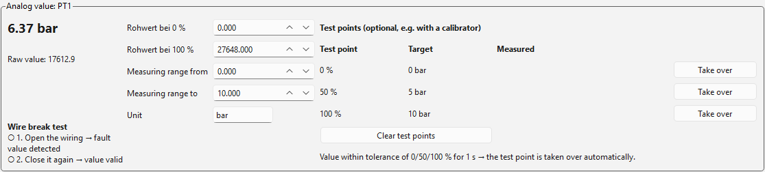
Analog value with wire break test and optional test points.
If an analog signal is selected, the Analog value box shows the scaled value, the raw value and fault values. The measuring range (raw value at 0 and 100 %, engineering range, unit) can be adjusted there.
Wire break test (analog inputs, the usual way): open the wiring of the signal (loosen the terminal) – the module reports a fault value, step 1 is checked – and close it again – the value is valid again, step 2 is checked. Then confirm the signal with ✓ OK or automatically with Check off signals automatically. If a different analog input than the selected one is interrupted, the swap warning appears. An interruption is a fault value (Siemens: above 32511, e.g. 32767; below −4864 with 4 … 20 mA, e.g. at 0 mA; −32768) or, with other raw ranges, a value more than 17.6 % outside. With 0 … 10 V and 0 … 20 mA an interruption cannot be distinguished from the value 0 – then check off by hand or use the test points.
Test points 0/50/100 % (optional, e.g. with a calibrator): if the value stays within the tolerance (toolbar, default 1 % of the measuring range) of a test point for 1 s, it is taken over – e.g. feed 4, 12 and 20 mA with a calibrator. Take over takes the current value by hand. When all three points are within tolerance, the signal becomes OK.
Fault values (Siemens raw values): 32767 = overflow or wire break, −32768 = underflow, 27649 … 32511 = overrange, below −4864 = underflow (wire break with 4 … 20 mA). With other raw ranges: value outside the measuring range.
Matrix and scanning ranges
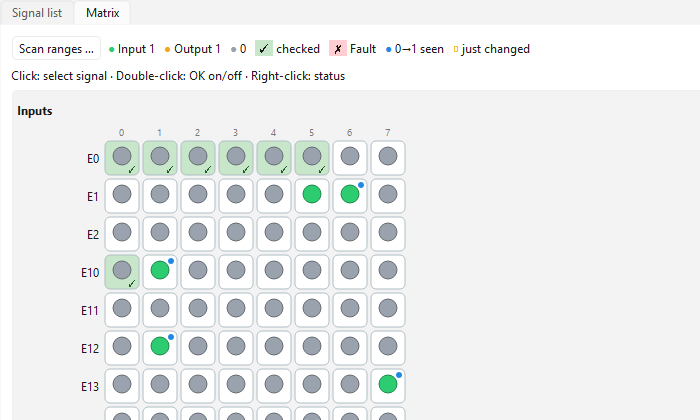
Matrix: inputs/outputs as LEDs, checked ones green with tick.
The Matrix tab shows all binary signals as LEDs: Siemens bit addresses by byte (row) and bit (column 0 … 7), separated into inputs, outputs and memory; other addresses in sequence.
LED green = input 1, orange = output 1, grey = 0, red = not readable.
Background green with ✓ = checked, red with ✗ = fault, grey with – = skipped. A blue dot means: 0→1 seen, but not yet 1→0 again. A yellow frame marks a change that has just happened, a blue frame the selected signal.
Click selects the signal (also in the list), double-click switches OK on/off, right-click opens the status selection; the tooltip shows symbol, comment, device tag and status.
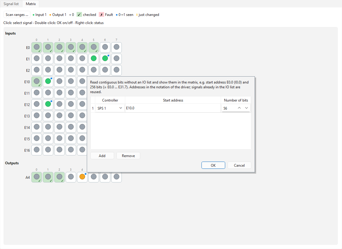
Scanning ranges without an IO list.
Scan ranges … reads contiguous bits also without an IO list, e.g. start address
E0.0 (I0.0) and 256 bits (= E0.0 … E31.7) or A0.0 (Q0.0) and 64 bits – useful
if there is no list yet. Addresses in the notation of the driver of the selected
controller; signals that are in the IO list keep their symbol and status. For s7
neighbouring addresses are read with one request per range.
Saving and result
Save stores the test progress as *.iocheck.json (signals, status, remarks, test
points, scan ranges, options). After the first save, every change is saved immediately –
you can stop at any time and continue the next day with Open …. Export result …
writes the list with status, check time, checker, remark and test points as Excel or CSV
file.
Checking on a smartphone or tablet
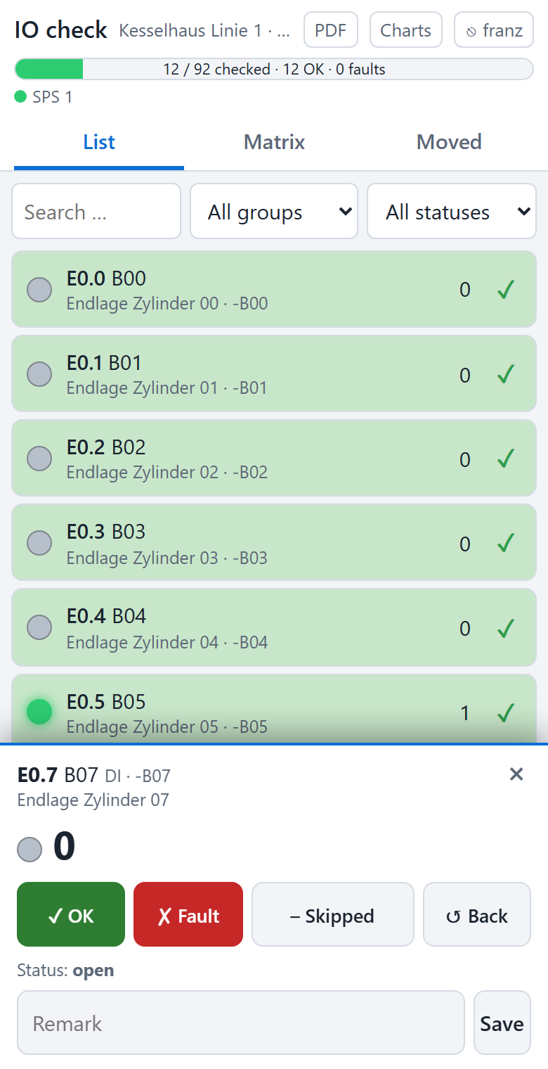
IO check on a smartphone: signal selected, status buttons at the bottom.
The technician at the machine sees live what arrives and checks off right there; several
devices can test at the same time. 📱 Mobile … in the toolbar shows the address (e.g.
https://192.168.0.20:8080/io) with a QR code for scanning and copies it to the
clipboard. If the web server is
already running in the logger, it is used (link IO-Check at the top of the chart page);
otherwise the IO check starts its own one with the settings of the configuration (tab
Web server & headless: port, HTTPS, users, access code; if the port is in use, the next
free one).
Tabs List (search, filter by group and status), Matrix (LEDs as on the PC) and Moved (latest changes). Tapping selects a signal; at the bottom the value, ✓ OK, ✗ Fault (with remark), Skipped, Back, the remark field and for analog inputs the wire break test and the test points appear (automatic take-over as on the PC while the signal is selected on the device).
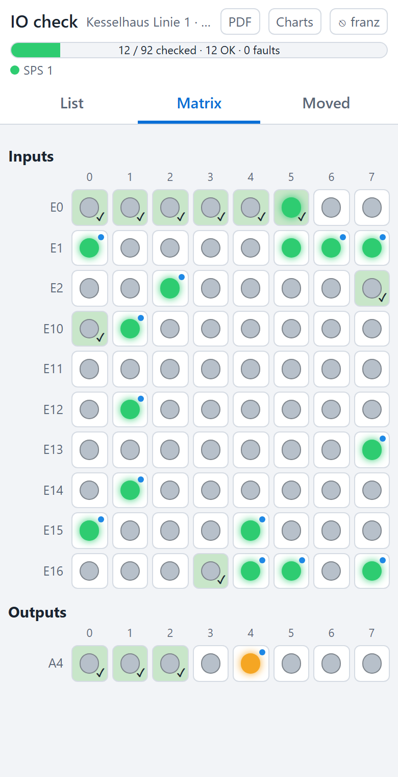
Matrix and swap warning on the smartphone.
The selected signal is expected on this device: if another digital input changes, the warning “Swapped?” appears and the device vibrates.
The checker is the login name in the web server (create users in the configuration program, see HTTPS and login); it appears in the list, the result and the protocol. Without login “Web (Zugriffscode)” or “Web (IP address)” is entered – then anybody in the network can change the status, so create users.
PDF at the top right opens the acceptance protocol on the device.
The IO check window on the PC takes over and saves the changes; it must stay open for this.
Acceptance protocol (PDF)
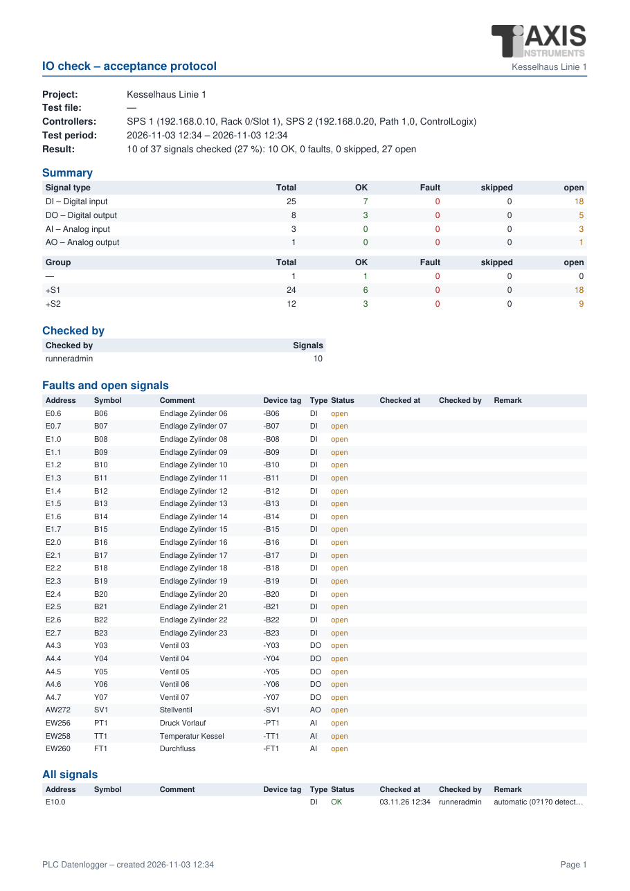
First page of an acceptance protocol.
Protocol (PDF) … creates the acceptance protocol and opens it:
Header: project, test progress file, controllers, test period and result (checked in %, OK, faults, skipped, open); above it the customer logo and logo of the configuration.
Summary per signal type and per group, checkers with the number of checked signals (PC user or login name in the web server).
Faults and open signals – the remaining items.
All signals per group with address, symbol, comment, device tag, type, status, check time, checker and remark or test points of the analog values.
Confirmation: signature fields for the checker and the acceptance (customer).
From scan ranges only edited signals appear. The protocol is created without additional programs (like the PDF reports); characters outside the Western European character set appear as “?”. The texts in the protocol follow the language of the program.
Switching and translating the language
The user interface is written in German and can be translated into other languages via language files. German and English are supplied.
Switching
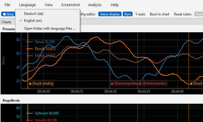
Menu Language.
Menu Language (in the logger and in the configuration program): choose the language
and confirm the restart question. The choice applies to both programs and the event
viewer and is stored in the file plc_einstellungen.json in the data folder. The
standard texts of Qt (Yes/No/Cancel, file dialogs) also follow the chosen language, and
Help › User manual (F1) opens the manual in the chosen language (English manual for
all languages except German).
Data is not translated: names of variables, charts and triggers, the columns of the CSV
files and of the event log (KOMMT, GEHT …), the keys of the configuration file,
the web page of the web server and (partly) the log file of headless operation.
Creating your own translation
Menu Language → Open folder with language files …. The folder
sprachenin the data folder opens; the templatede.txtis copied into it.Copy
de.txtand name it after the language code, e.g.fr.txt(French),it.txt,es.txt,nl.txt,pl.txt,cs.txt.Open the file with a text editor (UTF-8), enter the name after
# Sprache:at the top (e.g.Français) and write the translation after each>:# Sprache: Français @ Konfiguration laden > Charger la configuration @ {0} offene Ereignisse quittieren? > Acquitter {0} événements ouverts ?Save – the language appears immediately in the Language menu (active after a restart).
Rules:
@= German original text (do not change),>= translation. Translations left empty show the German text – so you can translate step by step.\nstands for a line break.Placeholders such as
{0},{1}or{2:.1f}must be kept (the order in the sentence is free). If one is missing, the original is used for this text.&in front of a letter marks the menu shortcut (Alt + letter);&&gives a single&.Leave HTML markup such as
<b>…</b>or<code>…</code>unchanged.The English file
en.txtcan serve as an example.
The program first looks in the folder sprachen of the data folder (own files, kept
during updates), then in the program folder (supplied files). An own en.txt in the
data folder therefore replaces the supplied one.
For developers: texts in the program are written as tr("…") or
tr("… {0} …").format(value) (module plc_i18n.py). After program changes
python tools/extract_tr.py plc . brings all language files up to date (new texts
with empty translation, existing translations are kept).
CSV files
File name and location
For each recording a new file is created in the CSV folder:
<CSV name>_YYYYMMDD_HHMMSS.csv, e.g. log_20261012_080000.csv (in demo mode
demo_...).
Limiting the file size and archiving
In the configuration the number of records per CSV file can be limited (Max. records
per file, 0 = unlimited). When the number is reached, the following happens
automatically:
The file is closed and zipped.
The ZIP is stored in the following folder structure:
<archive folder>/<CSV name>/<year>/<month>/<day>/<file name>.zip
Example:
archiv/log/2026/10/12/log_20261012_080000.zipThe original CSV file is only deleted after the archive has been checked successfully.
The recording continues without interruption in a new CSV file.
Notes:
Year, month and day are taken from the date of the first record of the file. The folder name
<CSV name>is the name set in the configuration (in demo modedemo).Zipping runs in the background and does not slow down the recording. The result appears in the status line. If archiving fails, the CSV file stays in the CSV folder.
If the recording is ended with ■ Stop, the current file stays unzipped in the CSV folder. Only full files are archived.
Archived files can be opened directly as ZIP with Load CSV.
The display in the logger works independently of the files; when a file is loaded, only its content is shown.
Rule of thumb for the file size: records per file = duration ÷ sampling interval. At an interval of 200 ms there are 5 records per second, i.e. 432,000 per day; a limit of 100,000 records then corresponds to about 5.5 hours per file.
Cleaning up old recordings
So that the disk or the database does not fill up, the logger can delete old recordings itself – by period (Delete after … days) and/or by storage space (Use at most … MB). Both limits are switched off by default (never or unlimited).
CSV and archive (tab Recording): only the files of this logger are affected –
<CSV name>_*.csvin the CSV folder and the ZIP files under<archive folder>/<CSV name>/. The decisive time is the last change of a file (= end of the recording in it). The CSV file currently being written is never deleted; archive folders that became empty are removed.Database (tab Database): values older than n days are deleted – row by row (in portions) for SQLite and MariaDB, whole chunks for TimescaleDB (
drop_chunks), whole daily partitions for QuestDB. The storage limit exists for SQLite only: if the values take up more than n MB, the oldest day is deleted at a time. The file does not get smaller, the freed space is reused for new values (to shrink it:VACUUMwith a SQLite tool). InfluxDB 3, VictoriaMetrics and Prometheus manage the retention period themselves (setting on the server).
The check runs when recording starts and then every hour, also in headless operation. What was deleted is shown in the status bar or the log (“[Clean-up] …”).
Warning
Deleted recordings cannot be restored. Choose the limits so that the data is kept as long as it is needed (e.g. retention obligations).
Format
Separator: semicolon (
;), decimal separator: pointCharacter set: UTF-8
First row: column headers
Column |
Content |
|---|---|
|
Timestamp with milliseconds, e.g. |
|
Unix time in seconds with three decimals (milliseconds), e.g.
|
Variables |
One column per variable, named after the variable. An empty field means: no valid value. |
Example:
Zeit;Epoch;Temperatur;Pumpe
2026-10-11 10:59:30.927;1791716370.927;51.234;1
2026-10-11 10:59:31.127;1791716371.127;51.301;1
Note
When the file is opened in Excel, Excel shows milliseconds only if the column is
formatted accordingly (custom number format yyyy-mm-dd hh:mm:ss.000). The values
in the file itself always contain the milliseconds.
Loading a CSV file
Load CSV opens one or more CSV or ZIP files (for ZIP archives the first CSV in the
archive) and shows them in offline mode; several files are joined by time (see below). A
running recording is stopped. The column Epoch is used for the display. Variables
whose name exists in the current configuration take over colour and assignment to chart
and Y axis; unknown variables appear on the first Y axis of the first chart.
Joining several CSV files
File › Join CSV files and save … chooses several recordings (CSV or archived ZIP
files, also from different archive folders) and joins them into one; the result is saved
as a new CSV file (suggestion: <CSV name>_<start>-<end>.csv) and shown offline.
The chosen files stay unchanged.
The order of the selection does not matter: all rows are sorted by time.
Columns are matched by variable name. If a variable is missing in a file (e.g. added later), it stays empty there.
Duplicate times (overlapping files) are taken over only once.
At gaps between the files (e.g. between two captures by trigger) an empty row is inserted so that the curves are interrupted there.
If you only want to view the files, simply choose them together in Load CSV – then without saving.
Exporting values (CSV/Excel)
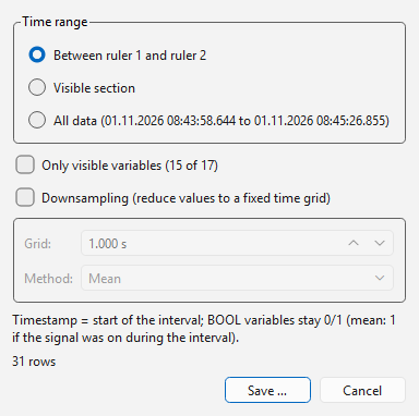
Dialog “Export values”.
File › Export values (CSV/Excel) … (Ctrl+Shift+E) saves measurements as CSV or
Excel file (.xlsx). The basis is the whole recording in memory or the loaded CSV
file or database time range.
Time range: Between ruler 1 and ruler 2 (offline only; the same data points as the statistics of the value table), Visible section or All data.
Only visible variables: hidden curves are left out.
Downsampling: reduces the values to a fixed time grid (e.g. 1 s or 60 s), e.g. to make long recordings smaller for Excel or a report. Method per interval: Mean, Minimum, Maximum, First value or Last value. The timestamp of a row is the start of its interval; intervals without data points are omitted. BOOL variables stay 0/1 (with the mean, 1 applies if the signal was on in the interval). The dialog shows how many rows will be created at most.
The format follows the file extension or the chosen file type:
CSV: same structure as the recording (
Zeit;Epoch;variables …, semicolon, decimal point) – the file can be opened again with Load CSV.Excel: column A date and time (with milliseconds), column B
Epoch, then one column per variable; missing values stay empty. A worksheet holds at most 1,048,575 rows – use downsampling or save as CSV for more data points.
Developing drivers
A driver is one Python file. It is loaded automatically at program start; the
program itself needs neither to be changed nor rebuilt – the installed .exe or the
AppImage also loads own drivers.
Where drivers are searched
Location |
Note |
|---|---|
Folder |
Recommended. Windows installed: |
Folders in the environment variable |
Separate several folders with |
Package |
File directly next to |
Files whose name starts with _ (e.g. _vorlage.py) are not loaded. Helper
modules of a driver can be placed next to it in the same folder (the folder is added to
the search path). If a driver cannot be loaded (syntax error, missing library on import,
duplicate ID), all others continue to work; the error message is shown under Driver ›
Installed drivers ….
Your own driver in five steps
Driver › Open folder for own drivers … – the folder then contains the template
_vorlage.py.Copy the template, e.g. to
my_plc.py(without_at the beginning). Unchanged, it is already a working driver “Simulation” that supplies sine, ramp, square and random values (addressessinus:20,rampe:10,rechteck:4,zufall:50).Adapt the ID
id(unique, stored in the configuration file),name,paramsandtypes.Fill
connect(),read()andclose()in the reader class with the protocol of the controller.Restart the configuration program – the driver appears in the Driver selection of the controller table.
Minimal driver
from plc_treiber.base import NAN, Driver, Param, Reader

class MyReader(Reader):
    def connect(self):
        # Establish the connection; report errors as exception (e.g. ConnectionError)
        self.sock = connect_to(self.plc.params["ip"], self.plc.params["port"])
        return len(self.vars)                 # number of readable variables

    def read(self):
        # ONE measurement cycle: values in the order of self.vars, float, NaN = no value
        out = []
        for v in self.vars:
            try:
                out.append(float(read_value(self.sock, v.address, v.dtype)))
                self.errors.pop(v.address, None)
            except KeyError as e:             # only this variable is missing
                self.errors[v.address] = str(e)
                out.append(NAN)
        return out

    def close(self):
        self.sock.close()

class MyDriver(Driver):
    id = "mine"
    name = "My controller"
    description = "Short description for the settings dialog"
    params = [
        Param("ip", "IP address", "text", "192.168.0.10"),
        Param("port", "Port", "int", 5000, minimum=1, maximum=65535),
    ]
    types = ["BOOL", "INT", "DINT", "REAL"]
    address_hint = "e.g. R100"

    def create_reader(self, plc, variables):
        return MyReader(self, plc, variables)

DRIVER = MyDriver()
Interface
All details are in src/plc_treiber/base.py. The most important parts:
Attribute |
Meaning |
|---|---|
|
Unique ID (lower case), stored as |
|
Display name (selection list) and description (settings dialog). |
|
List of |
|
Readable data types (choice from |
|
Label and tooltip texts for addresses and blocks. |
|
|
|
Text of the browse button; empty = no browse dialog. |
|
Name of the required library (for display). |
Method |
Task |
|---|---|
|
Returns the |
|
Short text of the connection for table, LEDs and messages. |
|
Error text for invalid parameters or |
|
Formal check of an address when saving; error text or |
|
Uniform notation (e.g. upper case). |
|
Address of the i-th block element ( |
|
Check of a block; size of a type in bytes (for display). |
|
Checks the library ( |
|
Connection test; default: |
|
Time of the controller as |
|
Browse dialog (Qt). |
Part |
Meaning |
|---|---|
|
Controller ( |
|
Establish and check the connection; return value: number of readable variables. |
|
One measurement cycle; list of |
|
Close the connection (may be called several times). |
|
|
Rules:
Report connection errors (controller not reachable, socket closed) as exception from
connect()/read(). The reading thread shows the LED red, closes the reader and reconnects after a short wait.Errors of single variables, on the other hand, are entered in
self.errorsand returnNAN– no exception.Each reader runs in its own thread; it does not need to be thread-safe, but must not share global objects with other readers without synchronization.
read()should take clearly less time than the interval of the controller.Texts for the user interface can be made translatable with
from plc_i18n import tr(tools/extract_tr.pyincludes drivers in the package).
For complete examples have a look at src/plc_treiber/modbus.py (own protocol via
sockets, combining requests, own address notation), src/plc_treiber/fins.py (own
protocol via UDP/TCP) and src/plc_treiber/s7.py (library, blocks, browse dialog).
Testing without user interface
import sys; sys.path.insert(0, r"C:\path\to\plc_datenlogger")
from plc_common import Plc, Variable
from plc_treiber import get_driver, load_errors

print(load_errors())                                  # load errors?
d = get_driver("mine")
plc = Plc(name="Test", driver="mine", params=d.default_params())
values, errors = d.read_once(plc, [Variable("A", address="R100", dtype="INT")])
print(values, errors)
Including a driver in the .exe
Own drivers in the folder treiber need no rebuild. If a driver is to be built in
permanently, put the file into plc_treiber/, enter its ID in BUILTIN in
src/plc_treiber/__init__.py (optional, only sets the order) and add required
libraries to requirements.txt and – if PyInstaller does not find them – as
--collect-all in build.bat or build_appimage.sh. build.bat includes all
modules of plc_treiber automatically (--collect-submodules plc_treiber).
Creating the setup file (Windows)
Three standalone programs (PLCLogger.exe, PLCKonfiguration.exe and
PLCIOCheck.exe) and a setup file can be created from the Python files. The following files are used:
File |
Task |
|---|---|
|
Builds both programs with PyInstaller into one common folder
( |
|
Inno Setup script (program folder, start menu, optional desktop icons, uninstallation, manual). |
|
Creates missing icon files ( |
|
Required Python packages (incl. PyInstaller and docutils for the build). |
Requirements: Python 3.9 or newer (64 bit), internet access on the first run (pip)
and, for the installer, Inno Setup 7 or 6 (https://jrsoftware.org/isinfo.php).
Procedure:
The folder structure of the project is kept (program files in
src, manual indoc, build files in the project folder; see overview).Start
build.batin the project folder (double-click or command prompt).build.bat everything: environment, programs, installer build.bat exe only the programs (dist\PLCDatenlogger) build.bat installer only the installer (requires an existing dist\) build.bat doc only the manual (HTML and PDF, German and English)
Result:
dist\PLCDatenlogger(runs without installation) andinstaller\PLCDatenlogger_Setup_<version>.exe.
The script creates a virtual environment .venv, installs the packages, creates the
icon if needed and builds both programs. The German manual (bedienungsanleitung.html)
and the English one (user_manual.html) are generated as well. The version number is
set at the top of build.bat under VERSION. Icon and logo are the files
app.ico and logo.png in the project folder; simply replace them to change them
(icon preferably with 256×256 pixels for a sharp symbol in Explorer and taskbar).
Data location: The installed programs do not write the configuration
(plc_config.json), CSV files and archive to the program folder (which is usually
write-protected), but to %APPDATA%\\PLCDatenlogger. The data is kept when
uninstalling and during updates. If everything is to be stored next to the programs
(portable operation on a USB stick), put an empty file portable.txt next to the
.exe files.
Notes:
The
.exefiles contain Python and all libraries (plctag.dlland the libraries of all built-in drivers – python-snap7, s7commplus, pycomm3, cryptography – are included; ifplctag.dllis missing next tobuild.bat, the script downloads it once from the GitHub release of libplctag); nothing has to be installed on the target computer.The logger starts the configuration via Config editor in the toolbar (
PLCKonfiguration.exein the same folder);PLCIOCheck.exeis the IO check as a program of its own (start menu PLC IO-Check).If the build fails, the cause is in the messages of the window (frequently: no internet for pip, Python not in PATH, virus scanner locks
dist). Withbuild.bat exethe steps can be repeated separately.
Portable version (without installation)
Instead of the installer, a ZIP package can be created that is only unpacked – e.g. onto a USB stick or into any folder:
build.bat portable
Result: dist\PLCDatenlogger_portable_<version>.zip (build.bat without parameter
creates the ZIP in addition to the installer). Usage:
Unpack the ZIP (right-click › Extract all).
Start
PLCKonfiguration.exeorPLCLogger.exein the unpacked folder. Neither an installation nor administrator rights are required.
The package contains the file portable.txt. It switches on portable operation:
configuration, CSV files, archive and log file are then stored in the unpacked
folder instead of under %APPDATA%. The folder must therefore be writable (so do
not unpack it under C:\Program Files). To remove the program, simply delete the
folder. For an update, unpack the new program files over the old folder; configuration
and recordings are kept.
Note
On the first start of a downloaded .exe Windows SmartScreen may warn (More info ›
Run anyway), because the programs are not signed. Via Properties › Unblock of the
ZIP file this can be lifted for all files before unpacking.
Building on GitHub (without a Windows PC of your own)
If the project is in a GitHub repository, the workflow .github/workflows/windows.yml
builds the portable ZIP and the installer on a Windows machine of GitHub:
Manually: Actions › Windows › Run workflow. The files are then in the summary of the run under Artifacts (
windows-portableandwindows-setup).With a tag
v*(e.g.v3.0.0): additionally as files of a GitHub release, together with the AppImages. The text of the release comes fromCHANGELOG.md.
The build uses build.bat as on your own PC. Images of the manual (folder
doc/images) are included if they are in the repository.
Version number: It is defined in exactly one place, APP_VERSION in
src/plc_common.py; build.bat, build_appimage.sh, the installer, the PDF manual
and the About dialog read it from there. The number follows the scheme
MAJOR.MINOR.PATCH (incompatible change / new features / bug fixes); the changes are
listed in CHANGELOG.md (German). New version and release:
python tools/bump_version.py minor --tag    # e.g. 3.0.0 -> 3.1.0: number, CHANGELOG, commit, tag
git push && git push origin v3.1.0          # push the tag: GitHub builds installer, ZIP and AppImages
If the tag does not match APP_VERSION, the workflow stops.
Automatic tests: the workflow .github/workflows/tests.yml runs on every push on
Linux and Windows: program logic, web server, notifications, OPC UA server, language
files and manual as well as the user interface with real PySide6 (without a screen).
Failures appear as annotations on the run. Locally:
pip install pytest
python -m pytest tests
Manual as PDF: This manual can be created as PDF with Sphinx – without LaTeX, via rinohtype:
pip install -r doc/requirements.txt
python tools/build_doc.py              # -> dist\PLC_Datenlogger_Bedienungsanleitung_<version>.pdf
python tools/build_doc.py --lang en    # -> dist\PLC_Datenlogger_User_Manual_<version>.pdf
python tools/build_doc.py --html       # additionally HTML preview in build\doc\html
It is easier with build.bat doc (Windows) or ./build_appimage.sh doc or
./build_macos.sh doc (Linux, macOS): the script creates a Python environment with the tools
if needed and builds only the manual – HTML (doc\*.html) and PDF in German and English
(build\doc\Bedienungsanleitung.pdf, User_Manual.pdf and copies with version number
in dist). On an error it shows the last messages; the complete ones are in
build\doc\pdf_de.log or pdf_en.log.
The settings are in doc/conf.py, the layout in doc/pdf.rtt (template) and
doc/pdf.rts (fonts, page breaks). The German manual is
doc/bedienungsanleitung.rst, the English one doc/user_manual.rst. The version
number comes from APP_VERSION in src/plc_common.py. build.bat creates the
PDFs automatically and puts them, in addition to the HTML manuals, into the installer
(start menu entries for the manual) and into the portable ZIP (folder Doku). If a PDF
fails, build.bat shows a note and continues without it.
Wiki: The workflow .github/workflows/wiki.yml regenerates the GitHub wiki with
every change of the manual (or of the images): one page per chapter, with sidebar and
images (tool tools/make_wiki.py, requires pandoc). Enable the wiki in the repository
once beforehand and create the first page. Do not edit the wiki pages by hand – they are
overwritten on the next run.
Linux: AppImage and Debian package (x86_64 and arm64)
For Linux the program is available as AppImage: a single file that runs without
installation. It contains the logger, the configuration program, the IO check and the event
viewer. Alternatively the same program is available as Debian package (.deb) for
Debian, Ubuntu, Linux Mint and Raspberry Pi OS, see Debian package.
Usage
chmod +x PLCDatenlogger-3.0.0-x86_64.AppImage        # once: make executable
./PLCDatenlogger-3.0.0-x86_64.AppImage               # logger (with start screen)
./PLCDatenlogger-3.0.0-x86_64.AppImage --konfig      # configuration program
./PLCDatenlogger-3.0.0-x86_64.AppImage --ereignisse  # event viewer
./PLCDatenlogger-3.0.0-x86_64.AppImage --headless plant.json   # recording only (e.g. as service)
On Raspberry Pi (64-bit system) and other arm64 computers use the file
…-aarch64.AppImage accordingly. The data (configuration, CSV, archive, events,
language files) is stored in ~/PLCDatenlogger; if a file portable.txt is next to
the AppImage, it stays in the folder of the AppImage. Some systems need the package
libfuse2 for AppImages (Ubuntu 22.04: sudo apt install libfuse2, Ubuntu 24.04:
libfuse2t64); without FUSE it also starts with --appimage-extract-and-run.
Wayland: On desktops with Wayland (e.g. Ubuntu, Fedora, KDE Plasma) all programs start
via XWayland. Under pure Wayland, Qt crashed when dragging a chart or value window
(dock); via XWayland the windows can also be moved and detached freely. An own
QT_QPA_PLATFORM still applies; with PLC_WAYLAND=1 the program runs under Wayland,
then the docks cannot be dragged (arrangement via the menu View). If XWayland is missing,
the same applies automatically.
The library libplctag (libplctag.so) is compiled from source during the build and
is contained in the AppImage.
Debian package (.deb)
The package installs the program permanently into the system, with start menu entries
(PLC Datenlogger, PLC Configuration, PLC IO check) and terminal commands. apt
installs the required system libraries (Qt graphics) along with it:
sudo apt install ./plc-datenlogger_3.2.1_amd64.deb   # PC (x86_64)
sudo apt install ./plc-datenlogger_3.2.1_arm64.deb   # Raspberry Pi 4/5 (64-bit system), arm64
plc-datenlogger                     # logger (with start screen)
plc-konfiguration                   # configuration program
plc-iocheck                         # IO check
plc-ereignisse                      # event viewer
plc-netzwerk                        # network panel for a touchscreen (Raspberry Pi)
plc-datenlogger --headless plant.json    # recording only (e.g. as service)
sudo apt remove plc-datenlogger     # remove (the data in ~/PLCDatenlogger is kept)
The program is installed in /usr/lib/PLCDatenlogger, the manual in
/usr/share/doc/PLCDatenlogger. As with the AppImage, the data is stored in
~/PLCDatenlogger (per user). An update is installed the same way with the newer .deb
file.
Which systems are suitable? As with the AppImage, the program needs at least the glibc of
the build system; apt checks this and refuses the package on systems that are too old:
amd64 (from the GitHub release): Ubuntu 22.04 and newer, Debian 12 and newer, Linux Mint 21 and newer.
arm64 (from the GitHub release): Raspberry Pi OS Bookworm and Trixie (64-bit), Ubuntu 22.04 and newer, Debian 12 and newer. A 32-bit Raspberry Pi OS is not supported (
dpkg --print-architecturemust showarm64). Up to version 3.4.0 the arm64 package needed Ubuntu 24.04 or Raspberry Pi OS Trixie.
Tried: Raspberry Pi with Ubuntu 24.04 (arm64, .deb from version 3.4.0) – controllers
with the drivers s7 and clx at the same time, with web server, with user interface and
in headless operation.
Setting up a Raspberry Pi as data logger
Step by step from an empty Raspberry Pi 4 (or 5) to continuous operation: logger without user interface as a service, values in VictoriaMetrics, display in the browser (the logger’s web server, Grafana). Everything is on an SSD on the USB 3 port – it copes with constant writing much better than an SD card.
Which system? Recommended: Ubuntu Server 24.04 LTS (64 bit) – the logger has been
tried on it, updates are available until 2029. The Pi boots without desktop; a desktop
(XFCE) only runs when needed via remote desktop (xrdp). On a connected touchscreen
the network panel shows the IP addresses and sets up Ethernet and WLAN (step 6).
Alternatives: Raspberry Pi OS Lite (64 bit, already includes NetworkManager) or DietPi (very
lean) – the .deb fits both, but the logger has not been tried there yet.
Hardware: Raspberry Pi 4 with at least 4 GB (2 GB are enough without remote desktop and Grafana), power supply 5.1 V/3 A, heat sink or fan, SSD in a USB 3 enclosure on a blue USB port, optionally a touchscreen (e.g. Waveshare, HDMI with USB touch or DSI).
1. Write the system directly to the SSD (on the PC, with the Raspberry Pi Imager):
Device Raspberry Pi 4, operating system Other general-purpose OS › Ubuntu › Ubuntu Server 24.04.x LTS (64-bit), storage: the SSD (connected to the PC via USB).
In the imager’s settings: host name (e.g.
logger-kessel), user and password, time zone, keyboard, enable SSH, WLAN if needed.Write, connect the SSD to the Pi, power on without SD card. A Pi 4 with a bootloader from September 2020 or later then boots from USB. If it does not: boot Raspberry Pi OS from an SD card once and run
sudo rpi-eeprom-update -a, and insudo raspi-configunder Advanced Options › Boot Order choose “USB Boot”.Log in:
ssh user@logger-kessel(or the IP address from the router). Check:findmnt -n -o SOURCE /shows/dev/sda2– the system runs from the SSD.
Variant: system on SD card, data on the SSD. Then mount the SSD at boot (caution: mkfs
erases the SSD):
lsblk                                        # find the SSD, e.g. /dev/sda1
sudo mkfs.ext4 -L daten /dev/sda1            # only for a new, empty SSD
sudo mkdir -p /data
echo 'LABEL=daten /data ext4 defaults,noatime,nofail,x-systemd.device-timeout=30 0 2' | sudo tee -a /etc/fstab
sudo systemctl daemon-reload && sudo mount -a && df -h /data
sudo mkdir -p /data/PLCDatenlogger && sudo chown $USER: /data/PLCDatenlogger
ln -s /data/PLCDatenlogger ~/PLCDatenlogger      # if ~/PLCDatenlogger exists already: see below
ls -l ~/PLCDatenlogger                           # shows -> /data/PLCDatenlogger
nofail makes sure the Pi also boots without SSD. The link puts the logger’s
configuration, CSV files, archive and log file on the SSD (the SD card wears out otherwise);
the VictoriaMetrics data follow in step 5. If ~/PLCDatenlogger exists already (the logger
has run before), stop the logger first and move the folder:
sudo systemctl stop plc-datenlogger              # or stop the headless logger in the configuration program
cp -a ~/PLCDatenlogger/. /data/PLCDatenlogger/
mv ~/PLCDatenlogger ~/PLCDatenlogger.alt
ln -s /data/PLCDatenlogger ~/PLCDatenlogger
sudo systemctl start plc-datenlogger
rm -r ~/PLCDatenlogger.alt                       # only once everything runs
The path ~/PLCDatenlogger/… stays the same – services and launchers need no change, only
the line RequiresMountsFor=/data in the logger’s service (step 4).
2. Basic setup:
sudo apt update && sudo apt full-upgrade -y && sudo reboot
timedatectl                                  # time zone and "System clock synchronized: yes"?
Time: the Pi 4 has no battery-backed clock. Without a time server the time is wrong after a power failure – and with it the time stamps. In a plant network without internet, enter a reachable time server (
/etc/systemd/timesyncd.conf, lineNTP=192.168.0.1, thensudo systemctl restart systemd-timesyncd) or use an RTC module.Network via NetworkManager: the network panel (step 6) and
nmcliset up Ethernet and WLAN. Ubuntu Server uses systemd-networkd at first; switch over (preferably with keyboard and screen on the Pi, the SSH connection may drop):sudo apt install -y network-manager echo 'network: {config: disabled}' | sudo tee /etc/cloud/cloud.cfg.d/99-disable-network-config.cfg printf 'network:\n version: 2\n renderer: NetworkManager\n' | sudo tee /etc/netplan/01-network-manager.yaml sudo rm -f /etc/netplan/50-cloud-init.yaml sudo touch /etc/NetworkManager/conf.d/10-globally-managed-devices.conf sudo chmod 600 /etc/netplan/*.yaml && sudo netplan apply && sudo reboot
Afterwards Ethernet gets its address via DHCP; a fixed address in the controller network is set in the panel or with
nmcli(reconnect the WLAN from the imager in the panel):nmcli device # interfaces and connections sudo nmcli connection modify "Wired connection 1" ipv4.method manual \ ipv4.addresses 192.168.0.50/24 ipv4.gateway 192.168.0.1 ipv4.dns 192.168.0.1 sudo nmcli connection up "Wired connection 1"
3. Install the logger (adjust the version number):
VER=3.12.1
wget https://github.com/franzhefekranz/PLC_Logger/releases/download/v$VER/plc-datenlogger_${VER}_arm64.deb
sudo apt install ./plc-datenlogger_${VER}_arm64.deb
Create the configuration on the PC with the configuration program (controllers, variables,
tab Web server & headless: web server on, Headless mode on, tab Database: VictoriaMetrics, server
127.0.0.1, port 8428) and copy it to the Pi:
scp anlage.json user@logger-kessel:~/PLCDatenlogger/       # on the PC
plc-datenlogger ~/PLCDatenlogger/anlage.json     # on the Pi via SSH: test run, Ctrl+C stops
Whether the logger runs with or without user interface is decided by the option Headless
mode in the configuration. Without a graphical session (service, SSH) it always runs
headless; in the remote desktop (step 7) plc-datenlogger opens the user interface if the
option is off – stop the service first, otherwise two loggers read the same controllers.
4. Logger as a service – starts at power-on and again after a crash. File
/etc/systemd/system/plc-datenlogger.service (adjust the user name):
[Unit]
Description=PLC Datenlogger (headless)
After=network-online.target docker.service
Wants=network-online.target
# RequiresMountsFor=/data          # only with data on the SSD (step 1): start once it is mounted

[Service]
User=user
ExecStart=/usr/bin/plc-datenlogger /home/user/PLCDatenlogger/anlage.json
Restart=on-failure
RestartSec=10
TimeoutStopSec=60

[Install]
WantedBy=multi-user.target
sudo systemctl daemon-reload
sudo systemctl enable --now plc-datenlogger
systemctl status plc-datenlogger                 # running?
tail -f ~/PLCDatenlogger/plc_logger.log          # messages
sudo systemctl stop plc-datenlogger              # stop (the CSV file is closed cleanly)
Restart=on-failure only restarts after a crash – if the logger is stopped in the
configuration program (Headless operation) or with systemctl stop, it
stays off.
5. VictoriaMetrics and Grafana (Docker). VictoriaMetrics runs permanently and starts
again after every reboot; Grafana only when needed – the logger’s web server is there for
the live display (http://logger-kessel:8080):
sudo apt install -y docker.io docker-compose-v2 git curl
sudo usermod -aG docker $USER  # then log out and in again (ssh)
git clone --depth 1 https://github.com/franzhefekranz/PLC_Logger.git ~/plc-docker
cd ~/plc-docker/docker && cp .env.example .env
nano .env                     # set GRAFANA_PASSWORD, VM_RETENTION (e.g. 1y)
cp grafana-bei-bedarf.yml docker-compose.override.yml   # do not start Grafana automatically
docker compose up -d --no-deps victoriametrics
docker compose ps
--no-deps only starts VictoriaMetrics (without the other databases of the test
environment).
System on SD card, data on the SSD (variant from step 1): otherwise VictoriaMetrics stores
its data in a Docker volume on the SD card. This moves the data to /data:
Let Docker wait for the SSD – otherwise VictoriaMetrics may start after booting before the SSD is mounted and silently write to the SD card.
sudo systemctl edit dockerand enter between the comment lines:[Unit] RequiresMountsFor=/data
Folder instead of volume: add to
~/plc-docker/docker/docker-compose.override.yml(created above fromgrafana-bei-bedarf.yml;docker-compose.ymlstays unchanged,git pullkeeps working):services: grafana: restart: "no" victoriametrics: volumes: - /data/victoriametrics:/storage
Take existing data along (only if something has been recorded already) and restart:
docker compose stop victoriametrics
docker volume ls | grep victoria             # name, usually docker_victoriametrics-data
sudo mkdir -p /data/victoriametrics
sudo cp -a /var/lib/docker/volumes/docker_victoriametrics-data/_data/. /data/victoriametrics/
docker compose up -d --no-deps victoriametrics
docker inspect plc-victoriametrics --format '{{range .Mounts}}{{.Source}} -> {{.Destination}}{{end}}'
The last line must show
/data/victoriametrics -> /storage. Storage … in the configuration program shows whether the recordings are there; then delete the old volume:docker volume rm docker_victoriametrics-data.
Alternatively {"data-root": "/data/docker"} in /etc/docker/daemon.json moves Docker
completely to the SSD (with Grafana and the images; RequiresMountsFor is needed then as
well).
Start and stop Grafana:
~/plc-docker/docker/grafana.sh start     # starts, waits until ready, opens the browser on the desktop
~/plc-docker/docker/grafana.sh stop      # stop (VictoriaMetrics keeps running)
~/plc-docker/docker/desktop-starter.sh   # once in the remote desktop: launchers "Grafana starten/beenden"
The launchers are then on the desktop and in the application menu of the remote desktop
session (step 7); without desktop, grafana.sh start via SSH and the browser on the PC
are enough. Grafana: http://logger-kessel:3000, the data source VictoriaMetrics is
already set up; upload the dashboard from File › Export Grafana dashboard … via
Dashboards › New › Import. After a reboot of the Pi, Grafana is off.
Accessing the database from the PC: VictoriaMetrics can be reached from the whole network (Docker publishes port 8428 on all interfaces of the Pi).
Logger on the PC (read mode): in the configuration, tab Database, enter the name or IP address of the Pi as server (
logger-kesselor192.168.0.50) instead of127.0.0.1; project and table as on the Pi. Then in the logger File › Load from database … (read mode). Simplest: the Pi’s name is already in the configuration running on the Pi – the logger there reaches itself that way too, and PC and Pi use the same file.Storage … in the configuration program shows the database usage on the Pi.
VictoriaMetrics web interface:
http://logger-kessel:8428/vmui.Grafana on the PC instead of on the Pi: data source of type Prometheus with the URL
http://logger-kessel:8428, then import the exported dashboard.
Securing it: VictoriaMetrics has no login – anyone in the network can read data, but also
write and delete. In an isolated control network this is usually fine, otherwise use one of
the two options (then docker compose up -d --no-deps victoriametrics):
Password: in
~/plc-docker/docker/docker-compose.ymladd to the servicevictoriametricsundercommand:- -httpAuth.username=logger - -httpAuth.password=secret
and enter user and password in the configuration program (tab Database) – on the Pi and on the PC; the logger then logs in with HTTP Basic. In Grafana switch on Basic auth for the data source (on the Pi under Connections › Data sources › VictoriaMetrics).
Publish to one network only: under
ports:prefix the Pi’s address in the desired network, e.g."192.168.0.50:8428:8428"instead of"8428:8428"(the logger on the Pi then also uses this address instead of127.0.0.1).
A firewall such as ufw does not help here: Docker adds published ports to the rules itself
and bypasses it.
6. Network panel on the touchscreen (plc-netzwerk): full screen, without desktop. It
shows host name, time, Ethernet and WLAN with IP addresses, the state of the logger service
and the address of the web server with a QR code (to open it on a tablet). The buttons
Ethernet and WLAN set DHCP or a fixed address (IP/prefix, gateway, DNS), search for
WLANs and connect with a password – input via the on-screen keyboard. The settings are kept
after a reboot. Next to the host name at the top the installed version is shown. ⏻ opens
the page Power off with Restart and Shut down (the logger service is stopped
properly); only unplug once the green LED has stopped blinking.
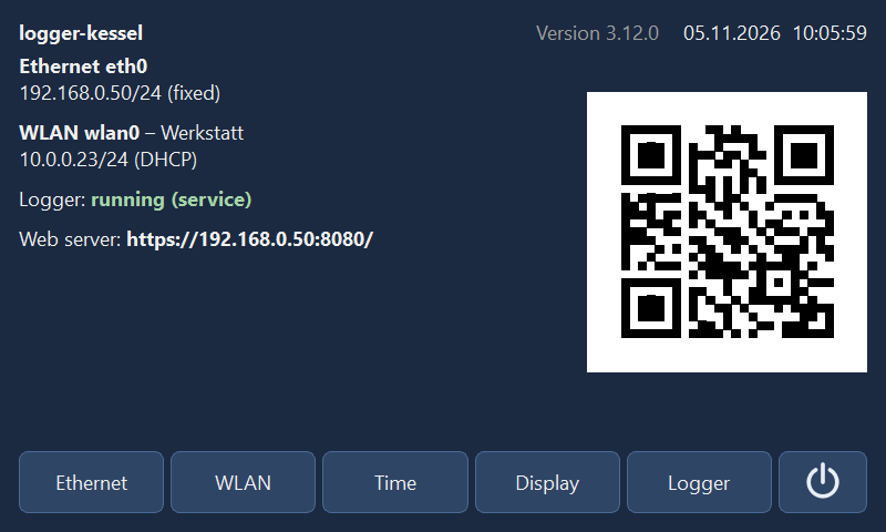
Network panel (800 × 480): overview with IP addresses, logger service and web server; at the top host name, installed version and time.
Logger lists the configuration files in the folder PLCDatenlogger (in the users’ home
folders and next to the file given at start) with their project name. Choose one and Start
(headless) – a logger that is already running is stopped first. If the service
plc-datenlogger (step 4) is set up, the panel switches it to the chosen file (drop-in
/etc/systemd/system/plc-datenlogger.service.d/konfig.conf), enables and restarts it – the
file then also starts after booting. Without the service the panel starts the logger directly
under the file’s owner, until the next reboot. Stop stops the logger and disables the
service. The web server address and the controller for the time then follow the chosen
configuration.
Page Logger: choose a configuration, start or stop it headless.
Display dims the screen after an adjustable time without touch (default 5 minutes,
0 = never); the first touch switches it on again without triggering a button and shows the
overview. Brightness in operation and in the dimmed state can also be set (0 % = backlight
off). This needs an adjustable backlight under /sys/class/backlight (present for DSI
displays with the dtoverlay according to the wiki, e.g. 10-0045); without it the
picture only turns black.
Page Display: time until dimming, brightness in operation and dimmed.
Time sets date and time – important because the Raspberry Pi 4 has no battery-backed clock and, without internet, starts with a wrong time after a reboot (the time stamps of the recording come from the Pi):
Manually: choose day, month, year, hour and minute with ▲/▼, Set clock. Internet time is switched off; Internet time (NTP) switches it on again. Time zone chooses the time zone from a list (e.g.
Europe/Berlin).From the controller: the row below appears when the configuration contains an active controller with the driver
s7,clxoropcua(with several, tapping the name selects the next one). Read shows the controller’s time and the difference to the Pi, Take over then sets the Pi.clx(system clock) andopcua(server time) deliver UTC; the panel converts to the Pi’s time zone. Withs7the CPU time is taken as local time; if the CPU clock runs in UTC (common with S7-1200/1500 – recognisable by a difference of whole hours), switch on UTC.tiacannot read the time; if PUT/GET is enabled in the CPU, an additional controller with the drivers7(same IP address) without variables is sufficient.Automatic: takes over the controller’s time when the panel starts and then every hour, as long as no internet time is synchronised and the difference is larger than 2 s (message on the overview). The panel’s settings are stored in
plc_netzwerk.jsonin root’s data folder.
Date and time: set manually or take over the time read from the controller.
Display: for Waveshare HDMI displays enter the lines for the respective model from the Waveshare wiki in
/boot/firmware/config.txt(resolution); touch works via USB without driver. DSI displays need thedtoverlayaccording to the wiki.Service
/etc/systemd/system/plc-netzwerk.service(runs as root because it changes the network; the configuration file only provides the web server address):[Unit] Description=PLC Datenlogger – Netzwerk-Panel (Touchscreen) After=NetworkManager.service Conflicts=getty@tty1.service [Service] ExecStart=/usr/bin/plc-netzwerk /home/user/PLCDatenlogger/anlage.json Restart=always RestartSec=5 [Install] WantedBy=multi-user.target
sudo systemctl daemon-reload && sudo systemctl enable --now plc-netzwerk“System policy prevents Wi-Fi scans” or no permission: the panel runs without root – e.g. started by hand without
sudoor via the desktop or xrdp. Best start it as a service (above) or withsudo plc-netzwerk --fenster. If it is to run as a normal user, a polkit rule allows the members of the groupnetdevto set network and time (file/etc/polkit-1/rules.d/50-plc-netzwerk.rules):polkit.addRule(function(action, subject) { if (subject.isInGroup("netdev") && (action.id.indexOf("org.freedesktop.NetworkManager.") == 0 || action.id.indexOf("org.freedesktop.timedate1.") == 0 || action.id.indexOf("org.freedesktop.login1.power-off") == 0 || action.id.indexOf("org.freedesktop.login1.reboot") == 0)) { return polkit.Result.YES; } });
sudo usermod -aG netdev benutzer # then log out and in againThis also allows Restart and Shut down. Switching the logger service (page Logger) still needs root.
Rotate the picture by 180°: add
Environment=QT_QPA_EGLFS_ROTATION=180. If the panel does not start (journalctl -u plc-netzwerk), addEnvironment=QT_QPA_PLATFORM=linuxfb. Without a graphics driver (no/dev/dri/card…) the panel useslinuxfbby itself. By hand (without service):sudo plc-netzwerk– on the text console, via SSH or from a terminal in the remote desktop, the panel always appears full screen on the Pi’s display (sudo timeout 600 plc-netzwerkends it after 10 minutes by itself). As a window in the remote desktop:sudo plc-netzwerk --fenster.
7. Remote desktop (XFCE and xrdp) – a desktop only when needed: the Pi keeps booting without user interface (the network panel runs on the display), and a remote desktop connection from the PC opens an XFCE session on the Pi.
a) Install the packages – with --no-install-recommends, otherwise xfce4 pulls in
the login screen lightdm, which would open the desktop on the Pi’s display at boot.
xorgxrdp is the graphics part of xrdp and therefore has to be listed explicitly:
sudo apt update
sudo apt install -y --no-install-recommends xfce4 xfce4-terminal xfce4-taskmanager \
     thunar mousepad dbus-x11 xrdp xorgxrdp fonts-dejavu adwaita-icon-theme
sudo snap install firefox                        # browser for Grafana (optional)
b) No desktop at boot – the Pi stays in text mode, even if a login screen gets installed later:
sudo systemctl set-default multi-user.target
systemctl get-default                            # must show multi-user.target
c) Set up xrdp – XFCE as the user’s session, access to the certificate, enable the service:
echo xfce4-session > ~/.xsession                 # for every user who logs in
sudo adduser xrdp ssl-cert
sudo systemctl enable --now xrdp
systemctl status xrdp                            # active (running)
d) Stop the “Authentication required” prompt – without this rule XFCE asks in the remote
session after every login for the password for a “color managed device” (colord). File
/etc/polkit-1/rules.d/45-xrdp-colord.rules:
polkit.addRule(function(action, subject) {
    if (action.id.indexOf("org.freedesktop.color-manager.") == 0 && subject.isInGroup("sudo")) {
        return polkit.Result.YES;
    }
});
e) Connect: on the PC connect to logger-kessel (port 3389) with Remote Desktop
Connection (Windows: mstsc, Linux: Remmina, macOS: Windows App), session Xorg, user
and password of the Pi. The configuration program, the logger’s user interface, the IO check
and Grafana in the browser (launchers from step 5) run there; File › Show/stop headless
loggers … sees the logger service because it runs under the same user. Logging out via the
XFCE menu ends the session; just closing the window keeps it running (the next connection
continues there).
If the window stays black after login or closes immediately: check ~/.xsession and look at
the messages (cat ~/.xsession-errors, sudo journalctl -u xrdp-sesman). The same user
must not be logged in graphically on the Pi’s display at the same time – which is not the case
here anyway because of multi-user.target.
Alternative Lubuntu (LXQt): looks like the logger’s programs (also Qt) but is much larger
(many additional programs, its own login screen sddm, which stays unused because of
multi-user.target); XFCE runs most reliably with xrdp. Instead of a) and the first line of
c):
sudo apt install -y lubuntu-desktop xrdp xorgxrdp
echo startlxqt > ~/.xsession
8. Operation:
Updates:
sudo apt update && sudo apt full-upgrade, a new logger with the newer.debfile, Docker:docker compose pull && docker compose up -d --no-deps victoriametrics(Grafana uses the new version at the nextgrafana.sh start).Check the space needed after a few hours with Storage … (tab Database).
Backup:
~/PLCDatenlogger(configuration, CSV) and the data folder of VictoriaMetrics (docker compose stop victoriametrics, copy the volume, start again).
Building
build_appimage.sh in the program folder builds the AppImage for the architecture of
the computer it runs on:
sudo apt install python3-venv cmake build-essential file libxkbcommon-x11-0 libxcb-cursor0 \
     libxcb-icccm4 libxcb-keysyms1 libxcb-shape0 libegl1 libfontconfig1 libdbus-1-3
./build_appimage.sh
# result: dist/PLCDatenlogger-3.0.0-x86_64.AppImage (or -aarch64)
#     and dist/plc-datenlogger_3.0.0_amd64.deb (or _arm64)
Build x86_64 on an x86_64 computer, arm64 on an arm64 computer (Raspberry Pi 4/5 with 64-bit system, Ubuntu arm64 …). PyInstaller cannot compile for another architecture.
Without an arm64 computer:
./build_appimage.sh --docker arm64builds in a Docker container via QEMU emulation (slow, but possible on any x86_64 PC with Docker).The AppImage runs on systems with the same or a newer glibc than the build system. For as many target systems as possible, build on an older system (e.g. Ubuntu 22.04).
If there is no suitable PySide6 package for an older arm64 system, use the Qt packages of the system:
sudo apt install python3-pyside6.qtwidgets python3-pyside6.qtsvgandVENV_SYSTEM=1 ./build_appimage.sh.The
.debpackage is created in the same run from the same program files (needsdpkg-deb, always present on Debian/Ubuntu);SKIP_DEB=1switches it off.GitHub Actions: The workflow
.github/workflows/appimage.ymlbuilds the AppImages and.debpackages for x86_64 and arm64 automatically if the project is in a GitHub repository (Actions › AppImages › Run workflow, or with a tagv*).
macOS (Apple Silicon and Intel)
For macOS the program is available as an app in a .dmg file:
PLCDatenlogger-<version>-macos-arm64.dmg for Macs with Apple Silicon (M1, M2 …) and
…-macos-x86_64.dmg for Intel Macs; both from macOS 12. The app contains the logger,
configuration program, IO check and event viewer, plus the manual and the PLC templates.
Note
The macOS version is a preview: it is built and tested automatically, but has not yet been operated on a Mac. Feedback (e.g. via GitHub) is welcome.
Installing: open the DMG and drag PLC Datenlogger onto Programme (Applications). The app is not signed and notarized by Apple; macOS therefore blocks it at the first start. Start it once in the Finder with right-click › Open and confirm (newer macOS versions: System Settings › Privacy & Security › Open Anyway) or in the terminal:
xattr -dr com.apple.quarantine "/Applications/PLC Datenlogger.app"
Usage: the app starts the logger with the start screen. The configuration program opens from the logger (config editor); parameters as under Linux:
"/Applications/PLC Datenlogger.app/Contents/MacOS/PLC Datenlogger" --konfig
"/Applications/PLC Datenlogger.app/Contents/MacOS/PLC Datenlogger" --headless plant.json
The data is stored in ~/PLCDatenlogger. As with Mac programs, the menu bar is at the top
of the screen; shortcuts with Ctrl use ⌘ on the Mac. libplctag (driver clx) is
included.
Building: build_macos.sh builds the app on a Mac for its architecture (needs Python
3.10+, the Xcode Command Line Tools and cmake for libplctag, e.g. brew install
cmake); result dist/PLC Datenlogger.app and the .dmg. The workflow
.github/workflows/macos.yml builds both variants on GitHub (Actions › macOS › Run
workflow, or with a tag v*) and attaches the .dmg files to the release. With an Apple
developer account the script signs with MACOS_SIGN_ID="Developer ID Application: …";
notarization then follows with xcrun notarytool.
Help and context help (F1)
Logger and configuration program have a Help menu:
User manual opens this manual (PDF or HTML) with the default program of the system. If the user interface is set to German, the German manual is opened, otherwise the English one.
About PLC Datenlogger … shows version, copyright, links to taxis-instruments.de and the source code on GitHub, the licence, the licences of the third-party components and the versions of the libraries used.
F1 opens the manual in the browser directly at the section that matches the current window – also in dialogs. The field with the input focus decides:
Configuration program: the matching section for each tab; in the controller table the section of the driver of the selected row; in the assignment tree, in the variable table and for the properties of chart and Y axis their section.
Dialogs: connection settings (section of the driver), select variables from the controller, blocks, calculated variables, triggers, PID controller, database read mode, event log, notes, web server users, XY chart, frequency analysis, IO check.
Logger: controls, charts, value table; start screen: section “Start screen”.
The context help needs the HTML version user_manual.html (German:
bedienungsanleitung.html; installer and portable version: subfolder Doku). If it
is missing, F1 opens the manual at the beginning.
Troubleshooting
Problem |
Possible cause and remedy |
|---|---|
“Connection failed” / LED red |
Check the connection parameters (… in the controller table) and the network
of the controller concerned, firewall ( |
“Library missing” in the settings dialog or under Installed drivers |
Install the library of the driver: |
Driver missing in the selection / “(driver missing)” |
Own driver not loaded: Driver › Installed drivers … shows the error message.
The file name must not start with |
|
DB too short or optimized block (offsets do not match) – create the block
without “Optimized block access” or use the driver |
|
TLS setting (try On or Off), password of the access level, number of free HMI connections of the CPU. |
|
Self-built program with Python 3.14 (e.g. WinPython 3.14, OpenSSL 3.5): use the
release files or build with Python 3.12 (delete |
|
In LOGO!Soft Comfort set up a connection as server with the matching TSAP
(default remote TSAP |
|
Put |
|
The tag does not exist (spelling, prefix |
|
Data file does not exist in the controller or is too short (e.g. |
|
Register not present in the device. Check the counting ( |
|
Check device address, baud rate, parity, stop bits; A/B line swapped? Bus termination present? Increase the timeout. |
|
Trust the client certificate in the server; choose the security as offered by the server. |
|
NodeId misspelled (namespace |
|
A route for the logger computer (AMS Net ID and IP address) must be entered in the TwinCAT controller; check the AMS Net ID and port (TwinCAT 3: 851, TwinCAT 2: 801) of the target. |
|
Check node numbers (network/node/unit) and UDP/TCP; with UDP the local node number must not be used by another device. |
|
Set up the connection in GX Works as binary; check series (Q/L or iQ-R), port and TCP/UDP. |
|
Device number outside the range of the CPU. |
|
Address out of range; address upper number ranges with |
|
Check adapter, interface, parity (even) and cabling; STEP 5 must not be connected at the same time. |
|
Wrong byte/word order (usually |
Browse dialog cannot be loaded |
Library of the driver missing (see above), check the connection. |
LED “Database” red |
Check server, port, database name and access data with Test database. The
database must exist ( |
Web page not reachable |
Web server switched on in the configuration? Port open in the firewall? Host
|
Browser warns about the certificate |
Normal for the self-signed certificate: compare the fingerprint (File › Web server address …) and confirm the exception, or use a certificate of the company CA. |
Logger starts without window |
Headless mode is active in the configuration. Start with |
Values are obviously wrong |
The set type does not match the variable (e.g. |
“No variables” at start |
First create and save variables in the configuration program, or use demo mode. |
No CSV file is written |
With Recording: By trigger with pre- and post-trigger time files are only created while the start condition is met (status bar ⏸ waiting for trigger). |
Changes to the configuration have no effect |
The logger loads the configuration at start. Press ■ Stop and ▶ Start again. |
Chart is empty |
Recording not running, or the variable is hidden via the tick in the value table. Check in the menu View › Pages / charts whether the chart is shown. |
Curve of a Y axis is not visible |
Fixed axis limits are outside the values. Activate Y auto or adjust the limits in the configuration. |
“⚠ Archiving … failed” |
Archive folder not writable or disk full. The CSV file stays in the CSV folder. |
Block cannot be read |
The range (start + count) does not completely exist in the controller, or the format does not match. Check size, index and format. |
Calculated variable shows no values |
Check the formula (editor: Check / calculate). Values that cannot be calculated result in gaps. At start the logger reports formula errors. |
Logo or icon does not appear |
Check the path in the configuration (relative paths refer to the program folder). Use PNG instead of SVG as an alternative (PDFs only support PNG and JPG). An empty logo field shows the manufacturer logo, “-” means “no logo”. |
Installed version does not find the configuration |
The data is stored under |
Single program can no longer read the file |
After saving in PLC Datenlogger the file has the new format (see Importing configurations of the single programs). Back up the old file beforehand with Save as…. |
No milliseconds in Excel |
Adjust the cell format (see note in the section CSV files). |
Known limitations
A block belongs to exactly one controller; formulas can, however, combine variables of different controllers (also of different drivers) – the latest value of each counts. The measurement times of the controllers are not synchronous.
Read-only access; the logger writes nothing to the controllers.
opcua: structures and strings cannot be recorded.s5as511: slow (9600 baud); read-only; data block addresses are determined when connecting.slmp,kvhostlink,toyopuc,s5as511,fins,adsandlogohave been tested against protocol simulators,pccconly with a simulated library; check with Test connection on the real controller before productive use.ads: only data types of fixed size (numbers, BOOL), no references/pointers and properties; a route in the controller is required.s7: only non-optimized blocks; names only via DB sources.tia: unofficial library; function depends on firmware and protection settings of the CPU.Numbers and
BOOLare recorded; strings and whole structures are not (their members are, though).A block has at most 1000 elements and exactly one format. If part of the range cannot be read, the whole block fails.
Own drivers run with the rights of the program; only put drivers from a trustworthy source into the driver folder.
The web server is read-only; without HTTPS unencrypted.
PDF reports use the standard font Helvetica: characters outside the Western European character set (Windows-1252) appear as “?”.
Automatic reports and recording by trigger refer to a running recording; after a restart the report period begins with the new data (partial report when stopping).
Calculated variables only know values of the current measurement (except
ddt,integandavg); when loading a CSV file they are taken from the file.Charts can only be rearranged by drag & drop within their page.
The minimum sampling time depends on the communication with the controller; with many variables the set interval may not be kept.
The demo switch and the window layout are not stored in the configuration file.
Licence
PLC Datenlogger · Copyright (C) 2026 Michael Taxis
The program is free software and is licensed under the GNU Lesser General Public
License, version 3 or (at your option) any later version (LGPL-3.0-or-later). It is
distributed in the hope that it will be useful, but without any warranty.
LICENSE– text of the GNU LGPL v3,COPYING– text of the GNU GPL v3, on which the LGPL v3 is based.THIRD_PARTY_LICENSES.md– licences of the supplied components: among others Qt/PySide6, asyncua and psycopg (LGPL-3.0), libplctag (MPL-2.0 or LGPL-2.0), the others under MIT, BSD or Apache-2.0.The files are in the program folder (portable version: also in the program folder, AppImage:
usr/share/doc). In the program Help › About PLC Datenlogger … shows version, licence and the libraries used.The libraries are separate files in the program folder (
_internal) and can be replaced by own, compatible versions.